
|
Архитектура Аудит Военная наука Иностранные языки Медицина Металлургия Метрология Образование Политология Производство Психология Стандартизация Технологии |
|
|
Архитектура Аудит Военная наука Иностранные языки Медицина Металлургия Метрология Образование Политология Производство Психология Стандартизация Технологии |
Distinction of Classes in the Feature Space⇐ ПредыдущаяСтр 85 из 85
Even if we take the best features available, there may be classes that can- not be separated. In such a case, it is always worth reminding us that separating the objects in well-defi ned classes is only a model of reality. Often, the transition from one class to another may not be abrupt but rather gradual. For example, anomalies in a cell may be present to a vary- 520 20 Classifi cation
Figure 20.6: Illustration of the recognition of letters with very similar shape such as the large ‘O’ and the fi gure ‘0’, or the letters ‘I’ and ‘l’ and the fi gure ‘1’.
ing degree, there not being two distinct classes, “normal” and “patho- logical”, but rather a continuous transition between the two. Thus, we cannot expect to fi nd well-separated classes in the feature space in every case. We can draw two conclusions. First, it is not guaranteed that we will fi nd well-separated classes in the feature space, even if optimal fea- tures have been selected. Second, this situation may force us to recon- sider the object classifi cation. Two object classes may either in reality be only one class or the visualization techniques to separate them may be inadequate. In another important application, optical character recognition, or OCR, we do have distinct classes. Each character is a well-defi ned class. While it is easy to distinguish most letters, some, e. g., the large ‘O’ and the fi gure ‘0’, or the letters ‘I’ and ‘l’ and the fi gure ‘1’, are very similar, i. e., lie close to each other in the feature space (Fig. 20.6). Such well- defi ned classes that hardly diff er in their features, pose serious problems for the classifi cation task. How can we then distinguish the large letter ‘O’ from the fi gure ‘0’ or an ‘l’ from a capital ‘I’? We can give two answers to this question. First, the fonts can be redesigned to make letters better distinguishable from each other. Indeed, special font sets have been designed for automated character recognition. Second, additional information can be brought into the classifi cation process. This requires, however, that the classifi cation does not stop at the level of individual letters; it must be advanced to the word level. Then, it is easy to establish rules for better recognition. One simple rule which helps to distinguish the letter ‘O’ from the fi gure ‘0’ is that letters and fi gures are not mixed in a word. As a counterexample to this rule, take British or Canadian zip codes which contain a blend of letters and fi gures. Anybody who is not trained to read this unusual mix has serious problems in reading and memorizing them. As another example, the capital ‘I’ can be distinguished from the lowercase ‘l’ by the rule that capital letters occur only as the fi rst letter in a word or in an all-capital-letter word. We close this section with the comment that asking whether a clas- sifi cation is at all possible for a given problem either by its nature or by the type of possible features is at least as important, if not more so, than the proper selection of a classifi cation method. 20.2 Feature Space 521
Principal Axes Transform The discussion in the previous section suggested that we must choose the object features very carefully. Each feature should bring in new in- formation which is orthogonal to what we already know about the ob- ject classes; i. e., object classes with a similar distribution in one feature should diff er in another feature. In other words, the features should be uncorrelated. The correlation of features can be studied with the statis- tical methods discussed in Section 3.3, provided that the distribution of the features for the diff erent classes is known (supervised classifi cation). The important quantity is the cross-covariance of two features mp and mq from the P-dimensional feature vector for one object class, which is defi ned as
(20.2)
is a measure for the variance of the feature. A good feature for a certain object class should show a small variance indicating a narrow extension of the cluster in the corresponding direction of the feature space. With P features, we can form a symmetric matrix with the coeffi cients Cpq, the covariance matrix C = C11 C12 ... C1, P C12 C22 ... C2, P
. (20.3) . . ... . C1, P C2, P... CP, P The diagonal elements of the covariance matrix contain the variances of the P features, while the off -diagonal elements constitute the cross- covariances. Like every symmetric matrix, the covariance matrix can be diagonalized (compare the discussion on the tensor representation of neighborhoods in Section 13.3). This procedure is called the principal- axes transform. The covariance matrix in the principal-axes coordinate system reads C1'1 0 ··· 0
0 C2'2 ... .
The diagonalization shows that we can fi nd a new coordinate system in which all features are uncorrelated. Those new features are linear 522 20 Classifi cation
Figure 20.7: Illustration of correlated features and the principal-axes transform.
combinations of the old features and are the eigenvectors of the covari- ance matrix. The corresponding eigenvalues are the variances of the transformed features. The best features show the lowest variance; fea- tures with large variances are not of much help since they are spread out in the feature space and, thus, do not contribute much to separating diff erent object classes. Thus, they can be omitted without making the classifi cation signifi cantly worse. A trivial but illustrative example is the case when two features are nearly identical, as illustrated in Fig. 20.7. In this example, the features m1 and m2 for an object class are almost identical, since all points in the feature space are close to the main diagonal and both features show a
a good feature, as it shows a narrow distribution, while m1' is as useless as m1 and m2 alone. Thus we can reduce the feature space from two dimensions to one without any disadvantages. In this way, we can use the principal-axes transform to reduce the dimension of the feature space and fi nd a smaller set of features which does nearly as good a job. This requires an analysis of the covariance matrix for all object classes. Only those features can be omitted where the analysis for all classes gives the same results. To avoid misunder- standings, the principal-axes transform cannot improve the separation quality. If a set of features cannot separate two classes, the same feature set transformed to the principal-axes coordinate system will not do so either. Given a set of features, we can only fi nd an optimal subset and, thus, reduce the computational costs of classifi cation. 20.3 Simple Classifi cation Techniques 523
20.2.6 Supervised and Unsupervised Classifi cation We can regard the classifi cation problem as an analysis of the struc- ture of the feature space. One object is thought of as a pattern in the feature space. Generally, we can distinguish between supervised clas- sifi cation and unsupervised classifi cation procedures. Supervision of a classifi cation procedure means determining the clusters in the feature space with known objects beforehand using teaching areas for identify- ing the clusters. Then, we know the number of classes and their location and extension in the feature space. With unsupervised classifi cation, no knowledge is presumed about the objects to be classifi ed. We compute the patterns in the feature space from the objects we want to classify and then perform an analysis of the clusters in the feature space. In this case, we do not even know the number of classes beforehand. They result from the number of well- separated clusters in the feature space. Obviously, this method is more objective, but it may result in a less favorable separation. Finally, we speak of learning methods if the feature space is updated by each new object that is classifi ed. Learning methods can compensate any temporal trends in the object features. Such trends may be due to simple reasons such as changes in the illumination, which could easily occur in an industrial environment because of changes in daylight, aging, or dirtying of the illumination system.
20.3 Simple Classifi cation Techniques In this section, we will discuss diff erent classifi cation techniques. They can be used for both unsupervised and supervised classifi cation. The techniques diff er only by the method used to associate classes with clus- ters in the feature space (Section 20.2.6). Once the clusters are identifi ed by either method, the further classi- fi cation process is identical for both of them. A new object delivers a feature vector that is associated with one of the classes or rejected as an unknown class. The diff erent classifi cation techniques diff er only by the manner in which the clusters are modeled in the feature space. Common to all classifi ers is a many to one mapping from the fea- ture space M to the decision space D. The decision space contains Q elements, each corresponding to a class including a possible rejection class for unidentifi able objects. In the case of a deterministic decision, the elements in the decision space are binary numbers. Then only one of the elemets can be one; all others must be zero. If the classifi ers gener- ates a probabilistic decision, the elements in the decision space are real numbers. Then the sum of all elements in the decision space must be one. 524 20 Classifi cation
20.3.1 Look-up Classifi cation This is the simplest classifi cation technique but in some cases also the best, since it does not perform any modeling of the clusters for the dif- ferent object classes, which can never be perfect. The basic approach of look-up classifi cation is very simple. Take the feature space as it is and mark in every cell to which class it belongs. Normally, a signifi cant amount of cells do not belong to any class and thus are marked with 0. In case the clusters from two classes overlap, we have two choices. First, we can take that class which shows the higher probability at this cell. Second, we could argue that an error-free classifi cation is not pos- sible with this feature vector and mark the cell with zero. After this initialization of the feature space, the classifi cation reduces to a simple look-up operation (Section 10.2.2). A feature vector m is taken and is looked up in the multidimensional look-up table to see which class, if any, it belongs to.
20.3.2 Box Classifi cation The box classifi er provides a simple modeling of the clusters in the fea- ture space. A cluster of one class is modeled by a bounding box tightly surrounding the area covered by the cluster (Fig. 20.8). It is obvious that the box method is a rather crude modeling. If we assume that the clus- ters are multidimensional normal distributions, then the clusters have an elliptic shape. These ellipses fi t rather well into the boxes when the axes of the ellipse are parallel to the axes of the feature space. In a two- dimensional feature space, for example, an ellipse with half-axes a and b has an area of π ab, the surrounding box an area of 4ab. This is not too bad. When the features are correlated with each other the clusters become long and narrow objects along diagonals in the feature space. Then the boxes contain a lot of void space and they tend much more easily to overlap, making classifi cation impossible in the overlapping areas. How- 20.3 Simple Classifi cation Techniques 525
0.2 0
Figure 20.8: Illustration of the box classifi er for the classifi cation of diff erent seeds from Fig. 20.2 into peppercorns, lentils, and sunfl ower seeds using the two features area and eccentricity.
Table 20.1: Parameters and results of the simple box classifi cation for the seeds shown in Fig. 20.2. The corresponding feature space is shown in Fig. 20.8.
ever, correlated features can be avoided by applying of the principal-axes transform (Section 20.2.5). The computations required for the box classifi er are still modest. For each class and for each dimension of the feature space, two compari- son operations must be performed to decide whether a feature vector belongs to a class or not. Thus, the maximum number of comparison operations for Q classes and a P-dimensional feature space is 2PQ. In contrast, the look-up classifi er required only P address calculations; the number of operations did not depend on the number of classes. To conclude this section we discuss a realistic classifi cation prob- lem. Figure 20.2 showed an image with three diff erent seeds, namely sunfl ower seeds, lentils, and peppercorns. This simple example shows many properties which are typical for a classifi cation problem. Although the three classes are well defi ned, a careful consideration of the features to be used for classifi cation is necessary since it is not immediately evi- 526 20 Classifi cation
A b
C d
Figure 20.9: Masked classifi ed objects from image Fig. 20.2 showing the classifi ed a peppercorns, b lentils, c sunfl ower seeds, and d rejected objects.
dent which parameters can be successfully used to distinguish between the three classes. Furthermore, the shape of the seeds, especially the sunfl ower seeds, shows considerable fl uctuations. The feature selection for this example was already discussed in Section 20.2.3. Figure 20.8 illustrates the box classifi cation using the two features area and eccentricity. The shaded rectangles mark the boxes used for the diff erent classes. The conditions for the three boxes are summa- rized in Table 20.1. As the fi nal result of the classifi cation, Fig. 20.9 shows four images. In each of the images, only objects belonging to one of the subtotals from Table 20.1 are masked out. From a total of 122 ob- jects, 103 objects were recognized. Thus 19 objects were rejected. They could not be assigned to any of the three classes for one of the following reasons:
20.3 Simple Classifi cation Techniques 527
0.2 0
0 200 400 600 800 1000 1200
Figure 20.10: Illustration of the minimum distance classifi er with the classifi - cation of diff erent seeds from Fig. 20.2 into peppercorns, lentils, and sunfl ower seeds using the two features area and eccentricity. A feature vector belongs to the cluster to which it has the minimal distance to the cluster center.
20.3.3 Minimum Distance Classifi cation The minimum distance classifi er is another simple way to model the clusters. Each cluster is simply represented by its center of mass mq. Based on this model, a simple partition of the feature space is given by searching for the minimum distance from the feature vector to each of the classes. To perform this operation, we simply compute the distance of the feature vector m to each cluster center mq: P
p=1 The feature is then assigned to the class to which it has the shortest distance. Geometrically, this approach partitions the feature space as illus- trated in Fig. 20.10. The boundaries between the clusters are hyper- 528 20 Classifi cation
planes perpendicular to the vectors connecting the cluster centers at a distance halfway between them. The minimum distance classifi er, like the box classifi er, requires a number of computations that is proportional to the dimension of the feature space and the number of clusters. It is a fl exible technique that can be modifi ed in various ways. The size of the cluster could be taken into account by introducing a scaling factor into the distance computation Eq. (20.5). In this way, a feature must be closer to a narrow cluster to be associated with it. Sec- ondly, we can defi ne a maximum distance for each class. If the distance of a feature is larger than the maximum distance for all clusters, the object is rejected as not belonging to any of the identifi ed classes.
20.3.4 Maximum Likelihood Classifi cation The maximum likelihood classifi er models the clusters as statistical prob- ability density functions. In the simplest case, P-dimensional normal distributions are taken. Given this model, we compute for each feature vector the probability that it belongs to any of the P classes. We can then associate the feature vector with the class for which it has the maximum likelihood. The new aspect with this technique is that probabilistic deci- sions are possible. It is not required that we decide to put an object into a certain class. We can simply give the object probabilities for member- ship in the diff erent classes.
20.4 Further Readings‡
From the vast amount of literature about classifi cation, we mention only three monographs here. The book of Schü rmann [166] shows in a unique the common concepts of classifi cation techniques based on classical statistical techniques and on neural networks. The application of neural networks for classifi cation is detailed by Bishop [9]. One of the most recent advances in classifi cation, the so-called support vector machines, are very readably introduced by Christianini and Shawe-Taylor [20].
Part V Reference Part
A Reference Material
Chip Format H × V
FR ID Pixel size H × V, µm
Comments
Interlaced EIA video Sony1 ICX258AL 768 × 494 30 6.09 6.35 × 7.4 1/3", eNIR Sony1 ICX248AL 768 × 494 30 8.07 8.4 × 9.8 1/2", eNIR
Sony1 ICX082AL 768 × 494 30 11.1 11.6 × 13.5 2/3" Interlaced CCIR video
Sony1 ICX259AL 752 × 582 25 6.09 6.5 × 6.25 1/3", eNIR Sony1 ICX249AL 752 × 582 25 8.07 8.6 × 8.3 1/2", eNIR
Sony1 ICX083AL 752 × 582 25 10.9 11.6 × 11.2 2/3" Progressive scanning interline
Sony1 ICX098AL 659 × 494 30 4.61 5.6 × 5.6 1/4" Sony1 ICX084AL 659 × 494 30 6.09 7.4 × 7.4 1/3" Sony1 ICX204AL 1024 × 768 15 5.95 4.65 × 4.65 1/3" Kodak2 KAI-0311M 648 × 484 30 7.28 9.0 × 9.0 1/2", QE 0.37 @ 500 nm
QE 0.43 @ 340 nm Sony1 ICX075AL 782 × 582 30 8.09 8.3 × 8.3 1/2" Sony1 ICX205AL 1360 × 1024 9.5 7.72 4.65 × 4.65 1/2", C 12 ke
QE 0.65 @ 500 nm
QE 0.54 @ 380 nm Kodak2 KAI-1020M 1000 × 1000 49 10.5 7.4 × 7.4 QE 0.45 @ 490 nm Kodak2 KAI-1010M 1008 × 1018 30 12.9 9.0 × 9.0 QE 0.37 @ 500 nm Kodak2 KAI-2000M 1600 × 1200 30 14.8 7.4 × 7.4 QE 0.36 @ 490 nm
Kodak2 KAI-4000M 2048 × 2048 15 21.4 7.4 × 7.4 QE 0.36 @ 490 nm 1 http: //www.sony.co.jp/en/Products/SC-HP/Product_List_E/index.html 2 http: //www.kodak.com/go/ccd
531 B. Jä hne, Digital Image Processing Copyright © 2002 by Springer-Verlag ISBN 3–540–67754–2 All rights of reproduction in any form reserved. 532 A Reference Material
Chip Format H × V
FR PC Pixel size H × V, µm
Comments
Linear response PhotonFocus1 640 × 480 30 10 10.5 × 10.5 32% fi ll factor
QE 0.22 @ 500 nm
Fast frame rate linear response
Photobit4 PB-MV13 1280 × 1024 600 80 12.0 × 12.0 10 parallel 10-bit ports
Photobit4 PB-MV02 512 × 512 4000 80 16.0 × 16.0 16 parallel 10-bit ports Logarithmic response
IMS HDRC VGA 5 640 × 480 25 8 12 × 12
light levels with ad- justable transition to logarithmic response 1 http: //www.photonfocus.com 2 http: //www.kodak.com/go/ccd 3 http: //www.fillfactory.com 4 http: //www.photobit.com 5 http: //www.ims-chips.de 533
Chip Format H × V
FR PC Pixel size H × V, µm
Comments
Near infrared (NIR) Indigo1 InGaAs 320 × 256 345 30 × 30 0.9–1.68 µm, C 3.5Me
1 http: //www.indogosystems.com 2 http: //www.aim-ir.de 3 http: //www.iaf.fhg.de/ir/qwip/index.html 534 A Reference Material
gˆ (k) = ∫ g(x) exp.− 2π ikTxΣ dW x =.exp.2π ikTxΣ .g(x).
s is a real, nonzero number, a and b are complex constants; A and U are W× W matrices, R is an orthogonal rotation matrix (R− 1 = RT, det R = 1) Property Spatial domain Fourier domain
Linearity ag(x) + bh(x) agˆ (k) + bhˆ (k) Similarity g(sx) gˆ (k/s)/|s| Generalized similarity g(Ax) gˆ.(A− 1)T kΣ / det A Rotation g(Rx)
gˆ (Rk)
Separability gw(xw) w=1 gˆ w(kw) w=1
T gˆ (k − k0)
Diff erentiation in x space ∂ g(x) ∂ xp
2π ikpgˆ (k)
Diff erentiation in k space ∂ g ˆ (k) − 2π ixpg(x) ∂ kp
Defi nite integral, mean ∫ g(x')dW x'
gˆ (0)
Moments ∫ xm
xng(x)dW x . i Σ m+n . ∂ m+ngˆ (k) Σ.
p q 2π
∂ km∂ kn
Convolution
Spatial correlation ∫ h(x')g(x − x')dW x' − ∞ ∫ h(x')g(x' + x)dW x' − ∞ hˆ (k)gˆ (k)
gˆ ∗ (k) hˆ (k) ∞ Multiplication h(x)g(x) ∞ ∫ hˆ (k')gˆ (k − k')dW k' − ∞ ∞ Inner product ∫ g∗ (x) h(x)dW x − ∞ ∫ gˆ ∗ (k)hˆ (k)dW k − ∞
535
2- Dand 3-Dfunctions are marked by † and ‡, respectively.
Space domain Fourier domain Delta, δ (x) const., 1 const., 1 Delta, δ (k)
− 1 x < 0
− i π k
π k
Disk, † 1
Π .|x| Σ Bessel, J1(2π r|k|)
2 Bessel, J 1 (2π x) x |k|3/(4π )
exp(− |x|), exp(− |x|)† 2 , 2π †
1 + (2π k)2 (1 + (2π |k|)2)3/2
Space domain Fourier domain
Gaussian, exp.− π xTxΣ Gaussian, exp.− π kTkΣ xp exp.− π xTxΣ − ikp exp.− π kTkΣ
exp(π x) + exp(− π x) sech(π k) 1
Hyperbola, |x|− W/2 |k|− W/2 ∞ ∞
536 A Reference Material
1 M− 1N− 1 gˆ u, v = MN.
. gm, nw− muw− nv, wN = exp (2π i/N) M N m=0n=0 M− 1N− 1 gm, n = . . gˆ u, v wmuwnv, M N u=0 v=0
Property Space domain Wave-number domain
Mean MN Gmn
gˆ 0, 0
Linearity aG + bH aGˆ + bHˆ
Spatial stretching (up- sampling) Replication (frequency stretching) gKm, Ln
gm, n (gkM+m, lN+n = gm, n) gˆ uv/(KL) (gˆ kM+u, lN+v = gˆ u, v ) gˆ Ku, Lv
gˆ u− u', v− v' Finite diff erences (gm+1, n − gm− 1, n)/2 (gm, n+1 − gm, n− 1)/2
i sin(2π u/M)gˆ uv i sin(2π v/N)gˆ uv Convolution . . hm'n' gm− m', n− n' MNhˆ uv gˆ uv m'=0n'=0 M− 1 N− 1 Spatial correlation . . hm'n' gm+m', n+n' MNhˆ uv gˆ u∗ v m'=0n'=0 M− 1 N− 1 Multiplication gmnhmn .. hu'v' gu− u', v− v'
Inner product Norm M− 1N− 1
|gmn|2 m=0n=0 u'=0v'=0 M− 1N− 1
|gˆ uv|2
537
hgˆ (k) =
with ∫ g(x) cas(2π kx)dx ◦ • g(x) =
∫ hgˆ (k) cas(2π kx)dk
cas 2π kx = cos(2π kx) + sin(2π kx). s is a real, nonzero number, a and b are real constants.
Property Spatial domain Fourier domain Linearity ag(x) + bh(x) agˆ (k) + bhˆ (k)
gˆ (k/s)/|s| Shift in x space g(x − x0) cos(2π kx0)gˆ (k)− sin(2π kx0)gˆ (− k) Modulation cos(2π k0x)g(x) .gˆ (k − k0) + gˆ (k + k0)Σ 2
Diff erentiation ∂ g(x) − 2π kpgˆ (− k) in x space
Defi nite integral, mean ∂ xp
− ∞
∞
gˆ (0) Convolution ∫ h(x')g(x − x')dx' [gˆ (k)hˆ (k) + gˆ (k)hˆ (− k) − ∞ +gˆ (− k)hˆ (k) − gˆ (− k)hˆ (− k)]/2 Multiplication h(x)g(x) [gˆ (k) ∗ hˆ (k) + gˆ (k) ∗ hˆ (− k) +gˆ (− k) ∗ hˆ (k) − gˆ (− k) ∗ hˆ (− k)]/2
− ∞
1. Fourier transform expressed in terms of the Hartley transform
gˆ (k) = 2 .hgˆ (k) +h gˆ (− k)Σ − 2 .hgˆ (k) − h gˆ (− k)Σ 2. Hartley transform expressed in terms of the Fourier transform h 1 i
gˆ (k) = ≡ [gˆ (k)] − ¥ [gˆ (k)] = 2 .gˆ (k) + gˆ ∗ (k)Σ + 2 .gˆ (k) − gˆ ∗ (k)Σ 538 A Reference Material
n!
n! (Q − n)! Continuous PDFs f (x) Uniform U(a, b) 1 b − a a + b
(b − a)2
12
Normal N(µ, σ ) 1
exp.− (x − µ)2 µ σ 2
Rayleigh R(σ ) x exp. x2 Σ , x > 0 σ , π /2 σ 2(4 − π )/2
σ 2 − 2σ 2
Chi-square χ 2(Q, σ )
2Q/2
Γ (Q/2)σ Q exp.− , x > 0 Qσ 2 2Qσ 4 2σ
Normal N(µ1, σ 1) N(µ2, σ 2) N(µ1 +µ2, (σ 2 + σ 2)1/2) 1 2
Chi-square χ 2(Q1, σ ) χ 2(Q2, σ ) χ 2(Q1 + Q2, σ ) PDFs of functions of independent random variables gn
gn: N(0, σ ) (g2 + g2)1/2 R(σ ) gn: N(0, σ ) arctan(g2/g2) U(0, 2π )
gn: N(0, σ ) 2 1 Q
χ 2(Q, σ )
n=1 539
matrix, and a a column vector with Q elements.
1. PDF, mean, and variance of a linear function g' = ag + b f '(g') = fg((g' − a)/b), µ ' = aµ
+ b, σ 2 = a2σ 2 g |a| g g g' g 2. PDF of monotonous diff erentiable nonlinear function g' = p(g)
' fg(p− 1(g')) fg'(g ) = dp(p− 1 ,
3. Mean and variance of diff erentiable nonlinear function g' = p(g) 2
µg' ≈ p(µg) + 2 g, σ g' ≈ g σ
4. Covariance matrix of a linear combination of RVs, g' = Mg + a cov(g') = M cov(g)MT 5. Covariance matrix of a nonlinear combination of RVs, g' = p(g)
6. Homogeneous stochastic fi eld: convolution of a random vector by the fi lter h g' = h ∗ g (Section 4.2.8) (a) With the autocovariance vector c
(b) With the autocovariance vector c = σ 2δ n (uncor.relate.d elements) 2 c' = σ 2(h > h) ◦ • c ˆ '(k) = σ 2 .h ˆ (k). .
. . 540 A Reference Material
1. Transfer function of a 1-D fi lter with an odd number of coeffi cients (2R + 1, [h− R,..., h− 1, h0, h1,..., hR]) (a) General hˆ (k˜ ) = R v'.=− R hv' exp(− π iv'k˜ ) (b) Even symmetry (h− v = hv)
hˆ v = h0 + 2 hv' cos(π v'k˜ ) v'=1 (c) Odd symmetry (h− v = − hv)
hˆ v = − 2i hv' sin(π v'k˜ ) v'=1 2. Transfer function of a 1-Dfi lter with an even number of coeffi cients (2R, [h− R,..., h− 1, h1,..., hR], convolution results put on intermedi- ate grid) (a) Even symmetry (h− v = hv)
hˆ v = 2 hv' cos(π (v' − 1/2)k˜ ) v'=1 (b) Odd symmetry (h− v = − hv)
hˆ v = − 2i hv' sin(π (v' − 1/2)k˜ ) v'=1 541
1. General fi lter equation
gn'
S
n''=1 R n'.=− R
hn' gn− n' 2. General transfer function
R
hˆ (k˜ ) = n'=− R
n''=0 3. Factorization of the transfer function using the z transform and the fundamental law of algebra
4. Relaxation fi lter
2R
S
n''=1 (a) Filter equation (|α | < 1) gn' (b) Point spread function
= α gn' ∓ 1 + (1 − α )gn
.(1 − α )α n n ≥ 0
(c) Transfer function of symmetric fi lter (running fi lter successively in positive and negative direction) rˆ (k˜ ) = 1 , .rˆ (0) = 1, rˆ (1) = 1 Σ
with 1 + β − β cos π k˜ 1 + 2β
(1 − α )2 β 542 A Reference Material
5. Resonance fi lter with unit response at resonance wave number k˜ 0 in the limit of low damping 1 − r, 1 (a) Filter equation (damping coeffi cient r ∈ [0, 1[, resonance wave number k˜ 0 ∈ [0, 1]) gn' = (1 − r 2) sin(π k˜ 0)gn + 2r cos(π k˜ 0)gn' ∓ 1 − r 2gn' ∓ 2 (b) Point spread function
(c) Transfer function of symmetric fi lter (running fi lter successively in positive and negative direction)
˜ sin2(π k˜ 0)(1 − r 2)2 sˆ (k) = ˜ ˜ 2 ˜ ˜ 2 .1 − 2r cos[π (k − k0)] + r Σ .1 − 2r cos[π (k + k0)] + r Σ (d) For low damping, the transfer function can be approximated by
for 1 − r, 1 (e) Halfwidth ∆ k, defi ned by sˆ (k˜ 0 + ∆ k) = 1/2 ∆ k ≈ (1 − r)/π
1. Construction of the Gaussian pyramid G(0), G(1),..., G(Q− 1) with Q planes by iterative smoothing and subsampling by a factor of two in all directions G(0) = G, G(q+1) = B↓ 2G(q) 2. Condition for smoothing fi lter to avoid aliasing
3. Construction of the Laplacian pyramid L(0), L(1),..., L(Q− 1) with Q planes from the Gaussian pyramid L(q) = G(q)− ↑ 2 G(q+1), L(Q− 1) = G(Q− 1) The last plane of the Laplacian pyramid is the last plane of the Gaussian pyramid.
4. Interpolation fi lters for upsampling operation ↑ 2 (± R22) 543 5. Iterative reconstruction of the original image from the Laplacian pyra- mid. Compute G(q− 1) = L(q− 1)+ ↑ 2 Gq
6. Directio-pyramidal decomposition in two directional components G(q+1) = ↓ 2 BxBy G(q) L(q) = G(q)− ↑ 2 G(q+1)
= 1/2(L(q) − (Bx = 1/2(L(q) + (Bx − By)G(q)) − By)G(q))
1. The frequency ν (cycles per unit time) and wavelength λ (length of a period) are related by the phase speed c (in vacuum speed of light c = 2.9979 × 10⁸ m s− 1): λ ν = c 2. Classifi cation of the ultraviolet, visible and infrared part of the elec- tromagnetic spectrum (see also Fig. 6.2)
544 A Reference Material
3. Energy and momentum of particulate radiation such as β radiation (electrons), α radiation (helium nuclei), neutrons, and photons (elec- tromagnetic radiation):
ν = E/h Bohr frequency condition, λ = h/p de Broglie wavelength relation.
dA0 is an element of area in the surface, θ the angle of incidence, Ω the solid angle. For energy-, photon-, and photometry-related terms, often the indices e, p, and ν, respectively, are used. Term Energy-related Photon-related Photometric quantity
[Ws] Photon number [1] Luminous energy [lm s] Energy fl ux (power)
Incident energy fl ux density
Excitant energy fl ux density
Energy fl ux per solid angle Radiant fl ux
dt Irradiance
dA0 Radiant excitance (emittance)
dA0 Radiant intensity
dΩ Photon fl ux [s− 1]
Photon irradi- ance [m− 2s− 1]
Photon fl ux density [m− 2s− 1]
Photon intensity [s− 1sr− 1] Luminous fl ux [lumen (lm)]
Illuminance [lm/m2 = lux [(lx)]
Luminous excitance [lm/m2]
Luminous intensity [lm/sr = candela (cd)] Energy fl ux density per solid angle Radiance
Photon radiance [m− 2s− 1sr− 1] Luminance [cd m− 2] [W m− 2 sr− 1] Energy/area Energy density [Ws m2]
Photon density [m− 2]
Exposure [lms m− 2 = lx s]
Computation of luminous quantities from the corresponding radiomet- ric quantity by the spectral luminous effi cacy V (λ ) for daylight (photopic) vision:
Q(λ )V(λ ) dλ 380 nm 545
Table with the 1980 CIE values of the spectral luminous effi cacy V (λ )
1. Human color vision based on three types of cones with maximal sen- sitivities at 445 nm, 535 nm, and 575 nm (Fig. 6.5b). 2. RGB color system; additive color system with the three primary col- ors red, green, and blue. This could either be monochromatic colors with wavelengths 700 nm, 646.1 nm, and 435.8 nm or red, green, and blue phosphor as used in RGB monitors (e. g., according to the Euro- pean EBU norm). Not all colors can be represented by the RGB color system (see Fig. 6.6a). 3. Chromaticity diagram: reduction of the 3-Dcolor space to a 2-Dcolor plane normalized by the intensity: r = R , g = G , b = B . R + G + B R + G + B R + G + B It is suffi cient to use the two components r and g: b = 1 − r − g. 4. XY Z color system (Fig. 6.6c): additive color system with three vir- tual primaries X, Y, and Z that can represent all possible colors and is given by the following linear transform from the EBU RGB color 546 A Reference Material
system: X 0.490 0.310 0.200 R
= 0.177 0.812 0.011 G
5. Color diff erence or YUV system: color system with an origin at the white point (Fig. 6.6b). 6. Hue-saturation (HSI) color system: color system using polar coordi- nates in a color diff erence system. The saturation is given by the radius and the hue by the angle.
1. Spectral emittance (law of Planck)
with Me(λ, T ) = 2π hc2
1
h = 6.6262 × 10− 34 J s Planck constant, kB = 1.3806 × 10− 23 J K− 1 Boltzmann constant, and c = 2.9979 × 10⁸ m s− 1 speed of light in vacuum. 2.
Me = 2 k4 π 5
T 4 = σ T 4 with σ ≈ 5.67 · 10− 8W m− 2K− 4 15 c2h3 3. Wavelength of maximum emittance (Wien’s law)
1. Snell’s law of refraction at the boundary of two optical media with the indices of refraction n1 and n2 sin θ 1 n2 sin θ 2 = n1 θ 1 and θ 2 are the angles of incidence and refraction, respectively. 2. Refl ectivity ρ: ratio of the refl ected radiant fl ux to the incident fl ux at the surface. Fresnel’s equations give the refl ectivity for parallel polarized light
ρ tan2(θ 1 − θ 2) ⊗ = tan2(θ 1 + θ 2), 547
for perpendicular polarized light
ρ
and for unpolarized light sin2(θ θ )
2 3. Refl ectivity at normal incidence (θ 1 = 0) for all polarization states
ρ (n1 − n2)2 (n − 1)2 = (n1 + n2)2 = (n + 1)2 with n = n1/n2 4. Total refl ection. When a ray enters into a medium with lower refrac- tive index, beyond the critical angle θ c all light is refl ected and none enters the optically thinner medium:
with n1 < n2
1. Perspective projection with pinhole camera model x1 d'X1
d'X2 2
Pinhole located at origin of world coordinate system [X1, X2, X3]T, d' is distance of image plane to projection center, X3 axis aligned perpendicular to image plane. 2. Image equation (Newtonian and Gaussian form) dd' = f 2 or 1 + 1 = 1 d' + f d + f f d and d' are the distances of the object and image to the front and back focal points of the optical system, respectively (see Fig. 7.7). 3. Lateral magnifi cation
ml = x1 f d'
4. Axial magnifi cation X1 = d = f
m d' f 2 d'2 2 a ≈ d = d2 = f 2 = ml 548 A Reference Material
5. The f -number nf of an optical system is the ratio of the focal length and diameter of lens aperture
2r 6. Depth of focus (image space)
7. Depth of fi eld (object space)
dmin
for range including infi nity dmin ≈
f 2
4nf H Microscopy (ml $ 1) ∆ X3 2nf H ≈ ml 8. Resolution with a diff raction-limited optical systems: angular reso- lution
na The resolution is given by the Rayleigh criterion (see Fig. 7.15b); na and na' are the object-sided and image sided numerical aperture of the light cone entering the optical system: na = n sin θ 0 = 2n = nr ; nf f n is the index of refraction. 9. Relation of the irradiance at image plane E' to the object radiance L (see Fig. 7.10)
E' =
2
f + d'
cos4 θ L ≈ tπ cos4 θ L for d f
549
Point operation that is independent of the position of the pixel Gm' n = P (Gmn) 1. Negative
PN(q) = Q − 1 − q 2.
3.
Puo (q) = (q − q1)(Q − 1) q ∈ [q1, q2]
Q − 1 q> q2
1.
If the variance of the noise depends on the image intensity, it can be equalized by a nonlinear grayscale transformation g g' = h(g)σ h∫ dg' + C
0 σ 2(g') with the two free parameters σ h and C. With a linear variance func- tion (Section 3.4.5) σ 2(g) = σ 2 + α g g the transformation becomes
0
σ 2 + α g + C. 2.
Two calibration images are taken, a dark image B without any illumi- nation and a reference image R with an object of constant radiance. A normalized image corrected for both the fi xed pattern noise and inhomogeneous sensitivity is given by
R − B 550 A Reference Material
1. Interpolation of continuous function from sampled points at dis- tances ∆ xw is an convolution operation: gr (x) =.n g(x n)h(x − x n). Reproduction of the grid points results in the interpolation condition
0 otherwise
2. Ideal interpolation function
h(x) =
W
w=1 hˆ (k) =
W
w=1 3.
Discrete 1-D interpolation fi lters for interpolation of intermediate grid points halfway between the existing points Type Mask Transfer function
Cubic − 1 9 9 − 1 /16 9 cos(π k/2) − cos(3π k/2) ˜ ˜ Cubic B-spline 1 23 23 1 /48 23 cos(π k/2) + cos(3π k/2)
3 16 + 8 cos(π k˜ )
†Recursive fi lter applied in forward and backward direction, see Section 10.6.5 551
1.
Summary of general constraints for averaging convolution fi lters Property Space domain Wave-number domain
hˆ (0) = 1
Zero shift, even symmetry h− n = hn ¥ .hˆ (k)Σ = 0 Monotonic decrease — from one to zero hˆ (k˜ 2) ≤ hˆ (k˜ 1) if k˜ 2 > k˜ 1, hˆ (k) ∈ [0, 1]
Isotropy h(x) = h(|x|) hˆ (k) = hˆ (|k|)
2.
1-Dsmoothing box fi lters Mask Transfer function Noise suppression†
3 1 2 ˜ 1 R = [1 1 1]/3 3 + 3 cos(π k) √ 3 ≈ 0.577
4R = [1 1 1 1]/4 cos(π k˜ ) cos(π k˜ /2) 1/2 = 0.5
2R+1R = [1 ... 1]/(2R + 1) sin(π (2R + 1)k˜ /2) √ 1
2RR = [1... 1]/(2R) (2R + 1) sin(π k˜ /2)
2R + 1 1
†For white noise
3.
1-Dsmoothing binomial fi lters Mask TF Noise suppression†
128 ≈ 0.523
1/4 2R 2R ˜ . Γ (R + 1/2) Σ
. 1 Σ . 1 Σ B †For white noise cos (π k/2) √ π Γ (R + 1) ≈ Rπ 1 − 16R 552 A Reference Material
1.
Summary of general constraints for a fi rst-order derivative fi lter into the direction xw Property Space domain Wave-number domain
hˆ (k ˜ ) .k˜ w =0 = 0 Zero shift, odd symmetry h− n = − hn ≡ .Hˆ (k)Σ = 0 First-order derivative .nwhn ∂ hˆ (k ˜ )
= π i
.k˜ w =0
Isotropy h(k) = π ikwb(.k.) with
.. 2. First-order discrete diff erence fi lters
Name Mask Transfer function
sin(π k˜ )
Cubic B-spline D2x ±R Σ 1 0 − 1 Σ /2, i x ˜ Σ 3 − √ 3, √ 3 − 2 Σ † 2/3 + 1/3 cos(π kx)
†Recursive fi lter applied in forward and backward direction, see Section 10.6.5 553
3.
Regularized fi rst-order discrete diff erence fi lters Name Mask Transfer function
2 × 2, D B 1 1 − 1
2i sin(π k˜ /2) cos(π k˜
/2)
1 1 0 –1
8 2 0 –2 1 0 –1 i sin(π k˜ x) cos2(π k˜ y /2) 1 3 0 –3
10 0 –10 3 0 –3 i sin(π k˜ x)(3 cos2(π k˜ y /2) + 1)/4
4.
Performance characteristics of edge detectors: angle error, magni- tude error, and noise suppression for white noise. The three values in the two error columns give the errors for a wave number range of 0–0.25, 0.25–0.5, and 0.5–0.75, respectively. Name Angle error [°] Magnitude error Noise factor
DxBy 0.67 2.27 5.10 0.013 0.079 0.221 1
y 554 A Reference Material
1.
Summary of general constraints for a second-order derivative fi lter into the direction xw Property Space domain Wave-number domain
hˆ (k ˜ ) .k˜ w
=0 = 0 Zero slope .nwhn ∂ hˆ (k ˜ ) = 0 ˜ . = 0 n ∂ kw .k˜ w =0 Zero shift, even symmetry h− n = hn ≡ .Hˆ (k)Σ = 0 Second-order derivative .n2 h 2 ∂ h(k). 2π 2
=−
Isotropy ˆ ˜ ˜ 2 ˆ ˜
.. 2. Second-order discrete diff erence fi lters
Name Mask Transfer function
Σ 1 − 2 1 Σ − 4 sin2(π k˜ x/2)
2-D Laplace L 0 1 0
− 4 sin (π kx/2)− 4 sin (π ky/2)
2-D Laplace L' 4 2 − 12 2 1 2 1 4 cos2(π kx/2) cos2(π ky/2) − 4
B Notation Because of the multidisciplinary nature of digital image processing, a consistent and generally accepted terminology — as in other areas — does not exist. Two basic problems must be addressed.
There exists no trivial solution to this awkward situation. Otherwise it would be available. Thus confl icting arguments must be balanced. In this textbook, the following guidelines are used:
In order to familiarize readers coming from diff erent backgrounds to the notation used in this textbook, we will give here some comments on deviating notations.
555 B. Jä hne, Digital Image Processing Copyright © 2002 by Springer-Verlag ISBN 3–540–67754–2 All rights of reproduction in any form reserved. 556 B Notation
λ and k 1 . (B.1) λ
Imaginary unit. The imaginary unit is denoted here by i. In electrical engineering and related areas, the symbol j is commonly used. Time series, image matrices. The standard notation for time series [133], x[n], is too cumbersome to be used with multidimensional signals: g[k][m][n]. Therefore the more compact notation xn and gk, m, n is chosen. Partial derivatives. In cases were it does not lead to confusion, partial derivates are abbreviated by indexing: ∂ g/∂ x = ∂ xg = gx
Typeface Description
e, i, d, w Upright symbols have a special √ meaning; examples: e for the base of natural logarithm, i = dg, w = e2π i a, b, … Italic (not bold): scalar − 1, symbol for derivatives: g, k, u, x, … Lowercase italic bold: vector, i. e., a coordinate vector, a time series, row of an image, … G, H, J, … Uppercase italic bold: matrix, tensor, i. e., a discrete image, a 2-Dconvolution mask, a structure tensor; also used for signals with more than two dimensions
N, Z, R, C Blackboard bold letters denote sets of numbers or other quan- tities
Accents Description
k ¯ , n ¯ , … A bar indicates a unit vector k˜, k ˜ , x ˜ , … A tilde indicates a dimensionless normalized quantity (of a quantity with a dimension)
G ˆ , gˆ (k), … A hat indicates a quantity in the Fourier domain 557
Subscript Description
gn Element n of the vector g gmn Element m, n of the matrix G gp Compact notation for fi rst-order partial derivative of the con- tinuous function g into the direction p: ∂ g(x)/∂ xp gpq Compact notation for second-order partial derivative of the continuous function g(x) into the directions p and q:
∂ 2g(x)/(∂ xp∂ xq)
Superscript Description
A− 1, A− g Inverse of a square matrix A; generalized inverse of a (non- square) matrix A AT Transpose of a matrix a> Conjugate complex
A> Conjugate complex and transpose of a matrix
Indexing Description
K, L, M, N Extension of discrete images in t, z, y, and x directions k, l, m, n Indices of discrete images in t, z, y, and x directions r, s, u, v Indices of discrete images in Fourier domain in t, z, y, and x directions P Number of components in a multichannel image; dimension of a feature space Q Number of quantization levels or number of object classes R Size of masks for neighborhood operators W Dimension of an image or feature space
p, q, w Indices of a component in a multichannel image, dimension in an image, quantization level or feature 558 B Notation
Function Description
cos(x) Cosine function exp(x) Exponential function ld(x) Logarithmic function to base 2 ln(x) Logarithmic function to base e log(x) Logarithmic function to base 10 sin(x) Sine function
sinc(x) Sinc function: sinc(x) = sin(π x)/(π x) det(G) Determinant of a square matrix
cov(g) Covariance matrix of a random vector
E(g), var(G) Expectation (mean value) and variance
Image operators Description
· Pointwise multiplication of two images ∗ Convolution > Correlation ∅, ⊕ Morphological erosion and dilation operators ◦ , • Morphological opening and closing operators ⊗ Morphological hit-miss operator ∨, ∧ Boolean or and and operators ∪, ∩ Union and intersection of sets ⊂, ⊆ Set is subset, subset or equal C Shift operator
559
Symbol Defi nition, [Units] Meaning
Greek symbols α [m− 1] Absorption coeffi cient β [m− 1] Scattering coeffi cient δ (x), δ n Continuous, discrete δ distribution W ∂ 2
∆ . ∂ x2 Laplacian operator w=1 w H [1] Specifi c emissivity H [m] Radius of blur disk κ [m− 1] Extinction coeffi cient, sum of absorp- tion and scattering coeffi cient
λ [m] Wavelength ν [s− 1], [Hz] (hertz) Frequency ∇ × Rotation operator η n + iξ, [1] Complex index of refraction η [1] Quantum effi ciency φ [rad], [°] Phase shift, phase diff erence φ e [rad], [°] Azimuth angle Φ [J/s], [W], [s− 1], [lm] Radiant or luminous fl ux Φ e, Φ p [W], [s− 1], [lm] Energy-based radiant, photon-based radiant, and luminous fl ux ρ, ρ ⊗ , ρ ⊥ [1] Refl ectivity for unpolarized, parallel polarized, and perpendicularly polar- ized light ρ [kg/m3] Density σ x Standard deviation of the random variable x σ 5.6696 · 10− 8Wm− 2K− 4 Stefan-Boltzmann constant σ s [m2] Scattering cross-section τ [1] Optical depth (thickness) τ [1] Transmissivity τ [s] Time constant θ [rad], [°] Angle of incidence θ b [rad], [°] Brewster angle (polarizing angle) θ c [rad], [°] Critical angle (for total refl ection) θ e [rad], [°] Polar angle θ i [rad], [°] Angle of incidence
continued on next page 560 B Notation
Symbol Defi nition, [Units] Meaning
continued from previous page Ω [sr] (steradian) Solid angle
ω ω = 2π ν, [s− 1], [Hz] Circular frequency Roman symbols
A [m2] Area a, a a = xtt = ut, [m/s2] Acceleration bˆ (k ˜ ) Transfer function of binomial mask B [Vs/m2] Magnetic fi eld B Binomial fi lter mask B Binomial convolution operator c 2.9979 · 108 ms− 1 speed of light C set of complex numbers d [m] Diameter (aperture) of optics, dis- tance d' [m] Distance in image space dˆ (k ˜ ) Transfer function of D D [m2/s] Diff usion coeffi cient D First-order diff erence fi lter mask D First-order diff erence operator e 1.6022 · 10− 19 As Elementary electric charge e 2.718281... Base for natural logarithm E [W/m2], [lm/m2], [lx] Radiant (irradiance) or luminous (illu- minance) incident energy fl ux density E [V/m] Electric fi eld e ¯ [1] Unit eigenvector of a matrix f, fe [m] (Eff ective) focal length of an optical system fb, ff [m] Back and front focal length f Optical fl ow f Feature vector F [N] (newton) Force G Image matrix H General fi lter mask h 6.6262 · 10− 34 Js Planck’s constant (action quantum) h h/(2π ) [Js] i I [W/sr], [lm/sr] Radiant or luminous intensity I [A] Electric current
continued on next page 561
Symbol Defi nition, [Units] Meaning
continued from previous page I Identity matrix I Identity operator J Structure tensor, inertia tensor kB 1.3806 · 10− 23 J/K Boltzmann constant k 1/λ, [m− 1] Magnitude of wave number k [m− 1] Wave number (number of wave- lengths per unit length) k˜ k∆ x/π Wave number normalized to the max- imum wave number that can be sam- pled (Nyquist wave number) Kq [l/mol] Quenching constant Kr Φ ν /Φ e, [lm/W] Radiation luminous effi ciency Ks Φ ν /P [lm/W] Lighting system luminous effi ciency KI [1] Indicator equilibrium constant L [W/(m2sr)], [1/(m2sr)], [lm/(m2sr)], [cd/m2] Radiant (radiance) or luminous (lumi- nance) fl ux density per solid angle L Laplacian fi lter mask L Laplacian operator m [kg] Mass m [1] Magnifi cation of an optical system m Feature vector M [W/m2], [1/(s m2)] Excitant radiant energy fl ux density (excitance, emittance) Me [W/m2] Energy-based excitance Mp [1/(s m2)] Photon-based excitance M Feature space n [1] Index of refraction na [1] Numerical aperture of an optical sys- tem nf f/d, [1] Aperture of an optical system n ¯ [1] Unit vector normal to a surface N Set of natural numbers: {0, 1, 2,...} p [kg m/s], [W m] Momentum p [N/m2] Pressure pH [1] pH value, negative logarithm of pro- ton concentration Q [Ws] (joule), [lm s] Radiant or luminous energy number of photons Qs [1] Scattering effi ciency factor
continued on next page 562 B Notation
Symbol Defi nition, [Units] Meaning
continued from previous page r [m] Radius T rm, n rm, n = Σ m∆ x, n∆ yΣ T Translation vector on grid r ˆ p, q r ˆ p, q = Σ p/∆ x, q/∆ yΣ Translation vector on reciprocal grid R Φ /s, [A/W] Responsivity of a radiation detector R Box fi lter mask R Set of real numbers s [A] Sensor signal T [K] Absolute temperature t [s] Time t [1] Transmittance u [m/s] Velocity u [m/s] Velocity vector U [V] Voltage, electric potential V [m3] Volume V (λ ) [lm/W] Spectral luminous effi cacy for pho- topic human vision V '(λ ) [lm/W] Spectral luminous effi cacy for sco- topic human vision w e2π i wN exp(2π i/N) T T x Σ x, yΣ , [x1, x2] Image coordinates in the spatial do- main X [X, Y, Z]T, [X1, X2, X3]T World coordinates
Z, Z+ Set of integers, positive integers
Bibliography [1] E. H. Adelson and J. R. Bergen. Spatio-temporal energy models for the perception of motion. J. Opt. Soc. Am. A, 2: 284–299, 1985. [2] E. H. Adelson and J. R. Bergen. The extraction of spatio-temporal en- ergy in human and machine vision. In Proceedings Workshop on Motion: Representation and Analysis, May 1986, Charleston, South Carolina, pp. 151–155. IEEE Computer Society, Washington, 1986. [3] A. V. Aho, J. E. Hopcroft, and J. D. Ullman. The Design and Analysis of Computer Algorithms. Addison-Wesley, Reading, MA, 1974. [4] J. Anton. Elementary Linear Algebra. John Wiley & Sons, New York, 2000. [5] G. R. Arce, N. C. Gallagher, and T. A. Nodes. Median fi lters: theory for one and two dimensional fi lters. JAI Press, Greenwich, USA, 1986. [6] S. Beauchemin and J. Barron. The computation of optical fl ow. ACM Computing Surveys, 27(3): 433–467, 1996. [7] L. M. Biberman, ed. Electro Optical Imaging: System Performance and Modeling. SPIE, Bellingham, WA, 2001. [8] J. Bigü n and G. H. Granlund. Optimal orientation detection of linear sym- metry. In Proceedings ICCV’87, London, pp. 433–438. IEEE, Washington, DC, 1987. [9] C. M. Bishop. Neural Networks for Pattern Recognition. Clarendon, Oxford, 1995. [10] R. Blahut. Fast Algorithms for Digital Signal Processing. Addison-Wesley, Reading, MA, 1985. [11] R. Bracewell. The Fourier Transform and its Applications. McGraw-Hill, New York, 2nd edn., 1986. [12] C. Broit. Optimal registrations of deformed images. Diss., Univ. of Penn- sylvania, USA, 1981. [13] H. Burkhardt, ed. Workshop on Texture Analysis, 1998. Albert-Ludwigs- Universitä t, Freiburg, Institut fü r Informatik. [14] H. Burkhardt and S. Siggelkow. Invariant features in pattern recognition - fundamentals and applications. In C. Kotropoulos and I. Pitas, eds., Non- linear Model-Based Image/Video Processing and Analysis, pp. 269–307. John Wiley & Sons, 2001. [15] P. J. Burt. The pyramid as a structure for effi cient computation. In A. Rosenfeld, ed., Multiresolution image processing and analysis, vol. 12 of Springer Series in Information Sciences, pp. 6–35. Springer, New York, 1984.
563 564 Bibliography
[16] P. J. Burt and E. H. Adelson. The Laplacian pyramid as a compact image code. IEEE Trans. COMM, 31: 532–540, 1983. [17] P. J. Burt, T. H. Hong, and A. Rosenfeld. Segmentation and estimation of image region properties through cooperative hierarchical computation. IEEE Trans. SMC, 11: 802–809, 1981. [18] J. F. Canny. A computational approach to edge detection. PAMI, 8: 679– 698, 1986. [19] R. Chelappa. Digital Image Processing. IEEE Computer Society Press, Los Alamitos, CA, 1992. [20] N. Christianini and J. Shawe-Taylor. An Introduction to Support Vector Machines. Cambridge University Press, Cambridge, 2000. [21] C. M. Close and D. K. Frederick. Modelling and Analysis of Dynamic Sys- tems. Houghton Miffl in, Boston, 1978. [22] J. W. Cooley and J. W. Tukey. An algorithm for the machine calculation of complex Fourier series. Math. of Comput., 19: 297–301, 1965. [23] J. Crank. The Mathematics of Diff usion. Oxford University Press, New York, 2nd edn., 1975. [24] P.-E. Danielsson, Q. Lin, and Q.-Z. Ye. Effi cient detection of second degree variations in 2D and 3D images. Technical Report LiTH-ISY- R-2155, Department of Electrical Engineering, Linkö ping University, S- 58183 Linkö ping, Sweden, 1999. [25] P. J. Davis. Interpolation and Approximation. Dover, New York, 1975. [26] C. DeCusaris, ed. Handbook of Applied Photometry. Springer, New York, 1998. [27] C. Demant, B. Streicher-Abel, and P. Waszkewitz. Industrial Image Process- ing. Viusal Quality Control in Manufacturing. Springer, Berlin, 1999. In- cludes CD-ROM. [28] P. DeMarco, J. Pokorny, and V. C. Smith. Full-spectrum cone sensitivity functions for X-chromosome-linked anomalous trichromats. J. of the Op- tical Society, A9: 1465–1476, 1992. [29] J. Dengler. Methoden und Algorithmen zur Analyse bewegter Realwelt- szenen im Hinblick auf ein Blindenhilfesystem. Diss., Univ. Heidelberg, 1985. [30] R. Deriche. Fast algorithms for low-level vision. IEEE Trans. PAMI, 12(1): 78–87, 1990. [31] N. Diehl and H. Burkhardt. Planar motion estimation with a fast converg- ing algorithm. In Proc. 8th Int. Conf. Pattern Recognition, ICPR’86, October 27–31, 1986, Paris, pp. 1099–1102. IEEE Computer Society, Los Alamitos, 1986. [32] R. C. Dorf and R. H. Bishop. Modern Control Systems. Addison-Wesley, Menlo Park, CA, 8th edn., 1998. [33] S. A. Drury. Image Interpretation in Geology. Chapman & Hall, London, 2nd edn., 1993. [34] M. A. H. Elmore, W. C. Physics of Waves. Dover Publications, New York, 1985. Bibliography 565
[35] A. Erhardt, G. Zinser, D. Komitowski, and J. Bille. Reconstructing 3D light microscopic images by digital image processing. Applied Optics, 24: 194– 200, 1985. [36] J. F. S. Crawford. Waves, vol. 3 of Berkely Physics Course. McGraw-Hill, New York, 1965. [37] O. Faugeras. Three-dimensional Computer Vision. A Geometric Vewpoint. MIT Press, Cambridge, MA, 1993. [38] M. Felsberg and G. Sommer. A new extension of linear signal process- ing for estimating local properties and detecting features. In G. Sommer, N. Krü ger, and C. Perwass, eds., Mustererkennung 2000, 22. DAGM Sym- posium, Kiel, Informatik aktuell, pp. 195–202. Springer, Berlin, 2000. [39] R. Feynman. Lectures on Physics, vol. 2. Addison-Wesley, Reading, Mass., 1964. [40] D. G. Fink and D. Christiansen, eds. Electronics Engineers’ Handbook. McGraw-Hill, New York, 3rd edn., 1989. [41] M. A. Fischler and O. Firschein, eds. Readings in Computer Vision: Issues, Problems, Principles, and Paradigms. Morgan Kaufmann, Los Altos, CA, 1987. [42] D. J. Fleet. Measurement of Image Velocity. Diss., University of Toronto, Canada, 1990. [43] D. J. Fleet. Measurement of Image Velocity. Kluwer Academic Publisher, Dordrecht, 1992. [44] D. J. Fleet and A. D. Jepson. Hierarchical construction of orientation and velocity selective fi lters. IEEE Trans. PAMI, 11(3): 315–324, 1989. [45] D. J. Fleet and A. D. Jepson. Computation of component image velocity from local phase information. Int. J. Comp. Vision, 5: 77–104, 1990. [46] J. D. Foley, A. van Dam, S. K. Feiner, and J. F. Hughes. Computer Graphics, Principles and Practice. Addison Wesley, Reading, MA, 1990. [47] W. Fö rstner. Image preprocessing for feature extraction in digital inten- sity, color and range images. In A. Dermanis, A. Grü n, and F. Sanso, eds., Geomatic Methods for the Analysis of Data in the Earth Sciences, vol. 95 of Lecture Notes in Earth Sciences. Springer, Berlin, 2000. [48] W. T. Freeman and E. H. Adelson. The design and use of steerable fi lters. IEEE Trans. PAMI, 13: 891–906, 1991. [49] G. Gaussorgues. Infrared Thermography. Chapman & Hall, London, 1994. [50] P. Geiß ler and B. Jä hne. One-image depth-from-focus for concentration measurements. In E. P. Baltsavias, ed., Proc. ISPRS Intercommission work- shop from pixels to sequences, Zü rich, March 22-24, pp. 122–127. RISC Books, Coventry UK, 1995. [51] J. Gelles, B. J. Schnapp, and M. P. Sheetz. Tracking kinesin driven move- ments with nanometre-scale precision. Nature, 331: 450–453, 1988. [52] F. Girosi, A. Verri, and V. Torre. Constraints for the computation of optical fl ow. In Proceedings Workshop on Visual Motion, March 1989, Irvine, CA, pp. 116–124. IEEE, Washington, 1989. [53] H. Goldstein. Classical Mechanics. Addison-Wesley, Reading, MA, 1980. 566 Bibliography
[54] G. H. Golub and C. F. van Loan. Matrix Computations. The John Hopkins University Press, Baltimore, 1989. [55] R. C. Gonzalez and R. E. Woods. Digital image processing. Addison-Wesley, Reading, MA, 1992. [56] G. H. Granlund. In search of a general picture processing operator. Comp. Graph. Imag. Process., 8: 155–173, 1978. [57] G. H. Granlund and H. Knutsson. Signal Processing for Computer Vision. Kluwer, 1995. [58] M. Groß. Visual Computing. Springer, Berlin, 1994. [59] E. M. Haacke, R. W. Brown, M. R. Thompson, and R. Venkatesan. Magnetic Resonance Imaging: Physical Principles and Sequence Design. John Wiley & Sons, New York, 1999. [60]
Advanced Imaging, Jan.: 46–48, 1996. [61] J. G. Harris. The coupled depth/slope approach to surface reconstruction. Master thesis, Dept. Elec. Eng. Comput. Sci., Cambridge, Mass., 1986. [62] J. G. Harris. A new approach to surface reconstruction: the coupled depth/slope model. In 1st Int. Conf. Comp. Vis. (ICCV), London, pp. 277– 283. IEEE Computer Society, Washington, 1987. [63] H. Hauß ecker. Messung und Simulation kleinskaliger Austauschvorgä nge an der Ozeanoberfl ä che mittels Thermographie. Diss., University of Hei- delberg, Germany, 1995. [64] H. Hauß ecker. Simultaneous estimation of optical fl ow and heat trans- port in infrared imaghe sequences. In Proc. IEEE Workshop on Computer Vision beyond the Visible Spectrum, pp. 85–93. IEEE Computer Society, Washington, DC, 2000. [65] H. Hauß ecker and D. J. Fleet. Computing optical fl ow with physical models of brightness variation. IEEE Trans. PAMI, 23: 661–673, 2001. [66] E. Hecht. Optics. Addison-Wesley, Reading, MA, 1987. [67] D. J. Heeger. Optical fl ow from spatiotemporal fi lters. Int. J. Comp. Vis., 1: 279–302, 1988. [68] E. C. Hildreth. Computations underlying the measurement of visual mo- tion. Artifi cial Intelligence, 23: 309–354, 1984. [69] G. C. Holst. CCD Arrays, Cameras, and Displays. SPIE, Bellingham, WA, 2nd edn., 1998. [70] G. C. Holst. Testing and Evaluation of Infrared Imaging Systems. SPIE, Bellingham, WA, 2nd edn., 1998. [71] G. C. Holst. Common Sense Approach to Thermal Imaging. SPIE, Belling- ham, WA, 2000. [72] G. C. Holst. Electro-optical Imaging System Performance. SPIE, Bellingham, WA, 2nd edn., 2000. [73] B. K. Horn. Robot Vision. MIT Press, Cambridge, MA, 1986. [74] S. Howell. Handbook of CCD Astronomy. Cambridge University Press, Cambridge, 2000. [75] T. S. Huang, ed. Two-dimensional Digital Signal Processing II: Transforms and Median Filters, vol. 43 of Topics in Applied Physics. Springer, New Bibliography 567
York, 1981. [76] S. V. Huff el and J. Vandewalle. The Total Least Squares Problem - Compu- tational Aspects and Analysis. SIAM, Philadelphia, 1991. [77] K. Iizuka. Engineering Optics, vol. 35 of Springer Series in Optical Sciences. Springer, Berlin, 2nd edn., 1987. [78] B. Jä hne. Image sequence analysis of complex physical objects: nonlinear small scale water surface waves. In Proceedings ICCV’87, London, pp. 191–200. IEEE Computer Society, Washington, DC, 1987. [79] B. Jä hne. Motion determination in space-time images. In Image Processing III, SPIE Proceeding 1135, international congress on optical science and engineering, Paris, 24-28 April 1989, pp. 147–152, 1989. [80] B. Jä hne. Spatio-temporal Image Processing. Lecture Notes in Computer Science. Springer, Berlin, 1993. [81] B. Jä hne. Handbook of Digital Image Processing for Scientifi c Applications. CRC Press, Boca Raton, FL, 1997. [82] B. Jä hne and H. Hauß ecker, eds. Computer Vision and Applications. A Guide for Students and Practitioners. Academic Press, San Diego, 2000. [83] B. Jä hne, H. Hauß ecker, and P. Geiß ler, eds. Handbook of Computer Vi- sion and Applications. Volume I: Sensors and Imaging. Volume II: Signal Processing and Pattern Recognition. Volume III: Systems and Applications. Academic Press, San Diego, 1999. Includes three CD-ROMs. [84] B. Jä hne, J. Klinke, and S. Waas. Imaging of short ocean wind waves: a critical theoretical review. J. Optical Soc. Amer. A, 11: 2197–2209, 1994. [85] B. Jä hne, H. Scharr, and S. Kö rgel. Principles of fi lter design. In B. Jä hne, H. Hauß ecker, and P. Geiß ler, eds., Computer Vision and Applications, vol- ume 2, Signal Processing and Pattern Recognition, chapter 6, pp. 125–151. Academic Press, San Diego, 1999. [86] A. K. Jain. Fundamentals of Digital Image Processing. Prentice-Hall, En- glewood Cliff s, NJ, 1989. [87] R. Jain, R. Kasturi, and B. G. Schunck. Machine Vision. McGraw-Hill, New York, 1995. [88] J. R. Janesick. Scientifi c Charge-Coupled Devices. SPIE, Bellingham, WA, 2001. [89] J. T. Kajiya. The rendering equation. Computer Graphics, 20: 143–150, 1986. [90] M. Kass and A. Witkin. Analysing oriented patterns. Comp. Vis. Graph. Im. Process., 37: 362–385, 1987. [91] M. Kass, A. Witkin, and D. Terzopoulos. Snakes: active contour models. In Proc. 1st Int. Conf. Comp. Vis. (ICCV), London, pp. 259–268. IEEE Computer Society, Washington, 1987. [92] B. Y. Kasturi and R. C. Jain. Computer Vision: Advances and Applications. IEEE Computer Society, Los Alamitos, 1991. [93] B. Y. Kasturi and R. C. Jain, eds. Computer Vision: Principles. IEEE Com- puter Society, Los Alamitos, 1991. [94] J. K. Kearney, W. B. Thompson, and D. L. Boley. Optical fl ow estimation: an error analysis of gradient-based methods with local optimization. IEEE 568 Bibliography
Trans. PAMI, 9 (2): 229–244, 1987. [95] M. Kerckhove, ed. Scale-Space and Morphology in Computer Vision, vol. 2106 of Lecture Notes in Computer Science, 2001. 3rd Int. Conf. Scale- Space’01, Vancouver, Canada, Springer, Berlin. [96] C. Kittel. Introduction to Solid State Physics. Wiley, New York, 1971. [97] R. Klette, A. Koschan, and K. Schlü ns. Computer Vision. Three-Dimensional Data from Images. Springer, New York, 1998. [98] H. Knutsson. Filtering and Reconstruction in Image Processing. Diss., Linkö ping Univ., Sweden, 1982. [99] H. Knutsson. Representing local structure using tensors. In The 6th Scan- dinavian Conference on Image Analysis, Oulu, Finland, June 19-22, 1989, 1989. [100] H. E. Knutsson, R. Wilson, and G. H. Granlund. Anisotropic nonstationary image estimation and its applications: part I – restoration of noisy images. IEEE Trans. COMM, 31(3): 388–397, 1983. [101] J. J. Koenderink and A. J. van Doorn. Generic neighborhood operators. IEEE Trans. PAMI, 14(6): 597–605, 1992. [102] C. Koschnitzke, R. Mehnert, and P. Quick. Das KMQ-Verfahren: Medi- enkompatible Ü bertragung echter Stereofarbabbildungen. Forschungs- bericht Nr. 201, Universitä t Hohenheim, 1983. [103] P. Lancaster and K. Salkauskas. Curve and Surface Fitting. An Introduction. Academic Press, London, 1986. [104] S. Lanser and W. Eckstein. Eine Modifi kation des Deriche-Verfahrens zur Kantendetektion. In B. Radig, ed., Mustererkennung 1991, vol. 290 of Informatik Fachberichte, pp. 151–158. 13. DAGM Symposium, Mü nchen, Springer, Berlin, 1991. [105] Laurin. The Photonics Design and Applications Handbook. Laurin Publish- ing CO, Pittsfi eld, MA, 40th edn., 1994. [106] D. C. Lay. Linear Algebra and Its Applications. Addison-Wesley, Reading, MA, 1999. [107] R. Lenz. Linsenfehlerkorrigierte Eichung von Halbleiterkameras mit Stan- dardobjektiven fü r hochgenaue 3D-Messungen in Echtzeit. In E. Paulus, ed., Proc. 9. DAGM-Symp. Mustererkennung 1987, Informatik Fachberichte 149, pp. 212–216. DAGM, Springer, Berlin, 1987. [108] R. Lenz. Zur Genauigkeit der Videometrie mit CCD-Sensoren. In H. Bunke, O. Kü bler, and P. Stucki, eds., Proc. 10. DAGM-Symp. Mustererkennung 1988, Informatik Fachberichte 180, pp. 179–189. DAGM, Springer, Berlin, 1988. [109] M. Levine. Vision in Man and Machine. McGraw-Hill, New York, 1985. [110] Z.-P. Liang and P. C. Lauterbur. Principles of Magnetic Resonance Imaging: A Signal Processing Perspective. SPIE, Bellingham, WA, 1999. [111] D. R. Lide, ed. CRC Handbook of Chemistry and Physics. CRC, Boca Raton, FL, 76th edn., 1995. [112] J. S. Lim. Two-dimensional Signal and Image Processing. Prentice-Hall, Englewood Cliff s, NJ, 1990. Bibliography 569
[113] T. Lindeberg. Scale-space Theory in Computer Vision. Kluwer Academic Publishers, Boston, 1994. [114] M. Loose, K. Meier, and J. Schemmel. A self-calibrating single-chip CMOS camera with logarithmic response. IEEE J. Solid-State Circuits, 36(4), 2001. [115] D. Lorenz. Das Stereobild in Wissenschaft und Technik. Deutsche Forschungs- und Versuchsanstalt fü r Luft- und Raumfahrt, Kö ln, Oberp- faff enhofen, 1985. [116] V. K. Madisetti and D. B. Williams, eds. The Digital Signal Processing Hand- book. CRC, Boca Raton, FL, 1998. [117] H. A. Mallot. Computational Vision: Information Processing in Perception and Visual Behavior. The MIT Press, Cambridge, MA, 2000. [118] V. Markandey and B. E. Flinchbaugh. Multispectral constraints for opti- cal fl ow computation. In Proc. 3rd Int. Conf. on Computer Vision 1990 (ICCV’90), Osaka, pp. 38–41. IEEE Computer Society, Los Alamitos, 1990. [119] S. L. Marple Jr. Digital Spectral Analysis with Applications. Prentice-Hall, Englewood Cliff s, NJ, 1987. [120] D. Marr. Vision. W. H. Freeman and Company, New York, 1982. [121] D. Marr and E. Hildreth. Theory of edge detection. Proc. Royal Society, London, Ser. B, 270: 187–217, 1980. [122] E. A. Maxwell. General Homogeneous Coordinates in Space of Three Di- mensions. University Press, Cambridge, 1951. [123] C. Mead. Analog VLSI and Neural Systems. Addison-Wesley, Reading, MA, 1989. [124] W. Menke. Geophysical Data Analysis: Discrete Inverse Theory, vol. 45 of International Geophysics Series. Academic Press, San Diego, 1989. [125] C. D. Meyer. Matrix Analysis and Applied Linear Algebra. SIAM, Philadel- phia, 2001. [126] A. Z. J. Mou, D. S. Rice, and W. Ding. VIS-based native video processing on UltraSPARC. In Proc. IEEE Int. Conf. on Image Proc., ICIP’96, pp. 153–156. IEEE, Lausanne, 1996. [127] T. Mü nsterer. Messung von Konzentrationsprofi len gelö ster Gase in der wasserseitigen Grenzschicht. Diploma thesis, University of Heidelberg, Germany, 1993. [128] H. Nagel. Displacement vectors derived from second-order intensity vari- ations in image sequences. Computer Vision, Graphics, and Image Process- ing (GVGIP), 21: 85–117, 1983. [129] Y. Nakayama and Y. Tanida, eds. Atlas of Visualization III. CRC, Boca Raton, FL, 1997. [130] V. S. Nalwa. A Guided Tour of Computer Vision. Addison-Wesley, Reading, MA, 1993. [131] M. Nielsen, P. Johansen, O. Olsen, and J. Weickert, eds. Scale-Space Theo- ries in Computer Vision, vol. 1682 of Lecture Notes in Computer Science, 1999. 2nd Int. Conf. Scale-Space’99, Corfu, Greece, Springer, Berlin. [132] H. K. Nishihara. Practical real-time stereo matcher. Optical Eng., 23: 536– 545, 1984. 570 Bibliography
[133] A. V. Oppenheim and R. W. Schafer. Discrete-time Signal Processing. Prentice-Hall, Englewood Cliff s, NJ, 1989. [134] A. Papoulis. Probability, Random Variables, and Stochastic Processes. McGraw-Hill, New York, 3rd edn., 1991. [135] J. R. Parker. Algorithms for Image Processing and Computer Vision. John Wiley & Sons, New York, 1997. Includes CD-ROM. [136] P. Perona and J. Malik. Scale space and edge detection using anisotropic diff usion. In Proc. IEEE comp. soc. workshop on computer vision (Miami Beach, Nov. 30-Dec. 2, 1987), pp. 16–20. IEEE Computer Society, Washing- ton, 1987. [137] Photobit. PB-MV13 20 mm CMOS Active Pixel Digital Image Sensor. Pho- tobit, Pasadena, CA, August 2000. www.photobit.com. [138] M. Pietikä inen and A. Rosenfeld. Image segmentation by texture using pyramid node linking. SMC, 11: 822–825, 1981. [139] I. Pitas. Digital Image Processing Algorithms. Prentice Hall, New York, 1993. [140] I. Pitas and A. N. Venetsanopoulos. Nonlinear Digital Filters. Principles and Applications. Kluwer Academic Publishers, Norwell, MA, 1990. [141] A. D. Poularikas, ed. The Transforms and Applications Handbook. CRC, Boca Raton, 1996. [142] W. Pratt. Digital image processing. Wiley, New York, 2nd edn., 1991. [143] W. H. Press, B. P. Flannery, S. A. Teukolsky, and W. T. Vetterling. Numerical Recipes in C: The Art of Scientifi c Computing. Cambridge University Press, New York, 1992. [144] J. G. Proakis and D. G. Manolakis. Digital Signal Processing. Principles, Algorithms, and Applications. McMillan, New York, 1992. [145] L. H. Quam. Hierarchical warp stereo. In Proc. DARPA Image Understand- ing Workshop, October 1984, New Orleans, LA, pp. 149–155, 1984. [146] A. R. Rao. A Taxonomy for Texture Description and Identifi cation. Springer, New York, 1990. [147] A. R. Rao and B. G. Schunck. Computing oriented texture fi elds. In Proceed- ings CVPR’89, San Diego, CA, pp. 61–68. IEEE Computer Society, Washing- ton, DC, 1989. [148] T. H. Reiss. Recognizing Planar Objects Using Invariant Image Features, vol. 676 of Lecture notes in computer science. Springer, Berlin, 1993. [149] J. A. Rice. Mathematical Statistics and Data Analysis. Duxbury Press, Belmont, CA, 1995. [150] A. Richards. Alien Vision: Exploring the Electromagnetic Spectrum with Imaging Technology. SPIE, Bellingham, WA, 2001. [151] J. A. Richards. Remote Sensing Digital Image Analysis. Springer, Berlin, 1986. [152] J. A. Richards and X. Jia. Remote Sensing Digital Image Analysis. Springer, Berlin, 1999. [153] M. J. Riedl. Optical Design Fundamentals for Infrared Systems. SPIE, Bellingham, 2nd edn., 2001. Bibliography 571
[154] K. Riemer. Analyse von Wasseroberfl ä chenwellen im Orts-Wellenzahl- Raum. Diss., Univ. Heidelberg, 1991. [155] K. Riemer, T. Scholz, and B. Jä hne. Bildfolgenanalyse im Orts- Wellenzahlraum. In B. Radig, ed., Mustererkennung 1991, Proc. 13. DAGM- Symposium Mü nchen, 9.-11. October 1991, pp. 223–230. Springer, Berlin, 1991. [156] A. Rosenfeld, ed. Multiresolution Image Processing and Analysis, vol. 12 of Springer Series in Information Sciences. Springer, New York, 1984. [157] A. Rosenfeld and A. C. Kak. Digital Picture Processing, vol. I and II. Acad- emic Press, San Diego, 2nd edn., 1982. [158] J. C. Russ. The Image Processing Handbook. CRC, Boca Raton, FL, 3rd edn., 1998. [159] H. Samet. Applications of Spatial Data Structures: Computer Graphics, Image processing, and GIS. Addison-Wesley, Reading, MA, 1990. [160] H. Samet. The Design and Analysis of Spatial Data Structures. Addison- Wesley, Reading, MA, 1990. [161] H. Scharr and D. Uttenweiler. 3D anisotropic diff usion fi ltering for en- hancing noisy actin fi laments. In B. Radig and S. Florczyk, eds., Pattern Recognition, 23rd DAGM Stmposium, Munich, vol. 2191 of Lecture Notes in Computer Science, pp. 69–75. Springer, Berlin, 2001. [162] H. Scharr and J. Weickert. An anisotropic diff usion algorithm with op- timized rotation invariance. In G. Sommer, N. Krü ger, and C. Perwass, eds., Mustererkennung 2000, Informatik Aktuell, pp. 460–467. 22. DAGM Symposium, Kiel, Springer, Berlin, 2000. [163] T. Scheuermann, G. Pfundt, P. Eyerer, and B. Jä hne. Oberfl ä chenkon- turvermessung mikroskopischer Objekte durch Projektion statistischer Rauschmuster. In G. Sagerer, S. Posch, and F. Kummert, eds., Muster- erkennung 1995, Proc. 17. DAGM-Symposium, Bielefeld, 13.-15. September 1995, pp. 319–326. DAGM, Springer, Berlin, 1995. [164] C. Schnö rr and J. Weickert. Variational image motion computations: the- oretical framework, problems and perspective. In G. Sommer, N. Krü ger, and C. Perwass, eds., Mustererkennung 2000, Informatik Aktuell, pp. 476– 487. 22. DAGM Symposium, Kiel, Springer, Berlin, 2000. [165] J. R. Schott. Remote Sensing. The Image Chain Approach. Oxford Univer- sity Press, New York, 1997. [166] J. Schü rmann. Pattern Classifi cation. John Wiley & Sons, New York, 1996. [167] R. Sedgewick. Algorithms in C, Part 1–4. Addison-Wesley, Reading, MA, 3rd edn., 1997. [168] J. Serra. Image analysis and mathematical morphology. Academic Press, London, 1982. [169] J. Serra and P. Soille, eds. Mathematical Morphology and its Applications to Image Processing, vol. 2 of Computational Imaging and Vision. Kluwer, Dordrecht, 1994. [170] E. P. Simoncelli, W. T. Freeman, E. H. Adelson, and D. J. Heeger. Shiftable multiscale transforms. IEEE Trans. IT, 38(2): 587–607, 1992. 572 Bibliography
[171] R. M. Simonds. Reduction of large convolutional kernels into multipass applications of small generating kernels. J. Opt. Soc. Am. A, 5: 1023–1029, 1988. [172] A. Singh. Optic Flow Computation: a Unifi ed Perspective. IEEE Computer Society Press, Los Alamitos, CA, 1991. [173] A. T. Smith and R. J. Snowden, eds. Visual Detection of Motion. Academic Press, London, 1994. [174] W. J. Smith. Modern Optical Design. McGraw-Hill, New York, 3rd edn., 2000. [175] P. Soille. Morphological Image Analysis. Principles and Applications. Springer, Berlin, 1999. [176] G. Sommer, ed. Geometric Computing with Cliff ord Algebras. Springer, Berlin, 2001. [177] J. Steurer, H. Giebel, and W. Altner. Ein lichtmikroskopisches Verfahren zur zweieinhalbdimensionalen Auswertung von Oberfl ä chen. In G. Hart- mann, ed., Proc. 8. DAGM-Symp. Mustererkennung 1986, Informatik- Fachberichte 125, pp. 66–70. DAGM, Springer, Berlin, 1986. [178] R. H. Stewart. Methods of Satellite Oceanography. University of California Press, Berkeley, 1985. [179] T. M. Strat. Recovering the camera parameters from a transformation matrix. In Proc. DARPA Image Understanding Workshop, pp. 264–271, 1984. [180] B. ter Haar Romeny, L. Florack, J. Koenderink, and M. Viergever, eds. Scale- Space Theory in Computer Vision, vol. 1252 of Lecture Notes in Computer Science, 1997. 1st Int. Conf., Scale-Space’97, Utrecht, The Netherlands, Springer, Berlin. [181] D. Terzopoulos. Regularization of inverse visual problems involving dis- continuities. IEEE Trans. PAMI, 8: 413–424, 1986. [182] D. Terzopoulos. The computation of visible-surface representations. IEEE Trans. PAMI, 10 (4): 417–438, 1988. [183] D. Terzopoulos, A. Witkin, and M. Kass. Symmetry-seeking models for 3D object reconstruction. In Proc. 1st Int. Conf. Comp. Vis. (ICCV), London, pp. 269–276. IEEE, IEEE Computer Society Press, Washington, 1987. [184] D. H. Towne. Wave Phenomena. Dover, New York, 1988. [185] S. Ullman. High-level Vision. Object Recognition and Visual Cognition. The MIT Press, Cambridge, MA, 1996. [186] S. E. Umbaugh. Computer Vision and Image Processing: A Practical Ap- proach Using CVIPTools. Prentice Hall PTR, Upper Saddle River, NJ, 1998. [187] M. Unser, A. Aldroubi, and M. Eden. Fast B-spline transforms for con- tinuous image representation and interpolation. IEEE Trans. PAMI, 13: 277–285, 1991. [188] F. van der Heijden. Image Based Measurement Systems. Object Recognition and Parameter Estimation. Wiley, Chichester, England, 1994. [189] W. M. Vaughan and G. Weber. Oxygen quenching of pyrenebutyric acid fl uorescence in water. Biochemistry, 9: 464, 1970. Bibliography 573
Addison-Wesley, Workingham, England, 1989. [195] J. Weickert. Anisotropic Diff usion in Image Processing. Dissertation, Fac- ulty of Mathematics, University of Kaiserslautern, 1996. [196] J. Weickert. Anisotrope Diff usion in Image Processing. Teubner, Stuttgart, 1998. [197] I. Wells, W. M. Effi cient synthesis of Gaussian fi lters by cascaded uniform fi lters. IEEE Trans. PAMI, 8(2): 234–239, 1989. [198] J. N. Wilson and G. X. Ritter. Handbook of Computer Vision Algorithms in Image Algebra. CRC, Boca Raton, FL, 2nd edn., 2000. [199] G. Wiora. Optische 3D-Messtechnik: Prä zise Gestaltvermessung mit einem erweiterten Streifenprojektionsverfahren. Dissertation, Fakultä t fü r Physik und Astronomie, Universitä t Heidelberg, 2001. http: //www.ub.uni-heidelberg.de/archiv/1808. [200] G. Wolberg. Digital Image Warping. IEEE Computer Society, Los Alamitos, CA, 1990. [201] R. J. Woodham. Multiple light source optical fl ow. In Proc. 3rd Int. Conf. on Computer Vision 1990 (ICCV’90), Osaka, pp. 42–46. IEEE Computer Society, Los Alamitos, 1990. [202] P. Zamperoni. Methoden der digitalen Bildsignalverarbeitung. Vieweg, Braunschweig, 1989. 574 Bibliography
Index Symbols 3- Dimaging 205 4- neighborhood 33 6-neighborhood 33 8-neighborhood 33
A absorption coeffi cient 170 accurate 77 acoustic imaging 153 acoustic wave 152 longitudinal 152 transversal 152 action quantum 150 action-perception cycle 16 active contour 442 active vision 16, 18 adder circuit 297 adiabatic compressibility 152 aerial image 514 AI 515 aliasing 233 alpha radiation 151 AltiVec 25 amplitude 56 amplitude of Fourier component 56 anaglyph method 210 analog-digital converter 247 analytic function 361 analytic signal 361 and operation 481 aperture problem 210, 379, 384, 385, 391, 394, 401, 450, 464 aperture stop 189 area 508 ARMA 116 artifi cial intelligence 18, 515 associativity 110, 484 astronomy 3, 18 autocorrelation function 94 autocovariance function 94 autoregressive-moving average process 116 averaging recursive 303 axial magnifi cation 187
B B-splines 276 back focal length 186 band sampling 156 band-limited 236 bandwidth-duration product 55 bandpass decomposition 135, 139 bandpass fi lter 121, 128 base orthonormal 39 basis image 39, 107 BCCE 386, 391 bed-of-nails function 236 Bessel function 199 beta radiation 151 bidirectional refl ectance distribution function 170 bimodal distribution 428 binary convolution 481 binary image 36, 427 binary noise 296 binomial distribution 89, 291 binomial fi lter 392 bioluminescence 173 bit reversal 68, 69 blackbody 163, 166 block matching 392 Bouger’s law 170 bounding box 499 box fi lter 286, 392 box function 196 BRDF 170 Brewster angle 169
575 576 Index
coherency radar 8, 218 coherent 150 color diff erence system 161 color image 283 cross-correlation function 95 cross-correlation spectrum 97 cross-covariance 521 cross-covariance function 95 Index 577
cyclic 343 cyclic convolution 105, 297 cyclic correlation 95
D data space 463 data vector 461, 468 decimation-in-frequency FFT 73 decimation-in-time FFT 68 decision space 523 deconvolution 113, 476 defocusing 474 deformation energy 450 degree of freedom 465 delta function, discrete 115 depth from multiple projections 208 phase 207 time-of-fl ight 207 triangulation 207 depth from paradigms 207 depth imaging 205, 206 depth map 6, 213, 441 depth of fi eld 188, 212, 477 depth of focus 187 depth range 208 depth resolution 208 depth-fi rst traversal 497 derivation theorem 53 derivative directional 358 partial 316 derivative fi lter 350 design matrix 461, 468 DFT 43 DHT 63 diff erence of Gaussian 335, 358 diff erential cross section 172 diff erential geometry 404 diff erential scale space 135, 139 diff erentiation 315 diff raction-limited optics 200 diff usion coeffi cient 129 diff usion equation 472 diff usion tensor 459 diff usion-reaction system 455 digital object 32 digital signal processing 77 digital video disk 24 digitization 15, 177, 233
dilation operator 482 direction 342 directional derivative 358 directiopyramidal decomposition 141, 411, 420 discrete convolution 102 discrete delta function 115 discrete diff erence 315 discrete Fourier transform 43, 116 discrete Hartley transform 63 discrete inverse problem 442 discrete scale space 136 disparity 209 dispersion 149 displacement vector 379, 385, 450 displacement vector fi eld 386, 442, 450 distance transform 493 distortion geometric 190 distribution function 79 distributivity 110, 485 divide and conquer 65, 72 DoG 335, 358 Doppler eff ect 174 dual base 242 dual operators 486 duality 486 DV 379, 385 DVD 24 DVD+RW 24 DVF 386 dyadic point operator 264, 320 dynamic range 208
E eccentricity 502 edge 308 in tree 435 edge detection 315, 323, 339 edge detector regularized 331 edge strength 315 edge-based segmentation 431 eff ective focal length 186 eff ective inverse OTF 478 effi ciency factor 172 eigenimage 114 eigenvalue 114, 459 eigenvalue analysis 400 578 Index
eigenvalue problem 346 eigenvector 114, 399 elastic membrane 450 elastic plate 451 elastic wave 152 elasticity constant 450 electric fi eld 147 electrical engineering 17 electromagnetic wave 147 electron 151 electron microscope 152 ellipse 502 elliptically polarized 150 emission 163 emissivity 165, 166 emittance 154 energy 58 ensemble average 93 ergodic 95 erosion operator 482 error calibration 77 statistical 77 systematic 77 error functional 446 error propagation 465 error vector 461 Ethernet 24 Euclidian distance 34 Euler-Lagrange equation 445, 455 excitance 154 expansion operator 139 expectation value 80 exponential, complex 114 exposure time 87 extinction coeffi cient 171
F fan-beam projection 224 Faraday eff ect 173 fast Fourier transform 66 father node 435 feature 99 feature image 15, 99, 339 feature space 517 feature vector 517 FFT 66 decimation-in-frequency 73 decimation-in-time 68 multidimensional 74 radix-2 decimation-in-time 66 radix-4 decimation-in-time 72 fi eld electric 147 magnetic 147 fi ll operation 500 fi lter 52, 99 binomial 290 causal 115 diff erence of Gaussian 358 fi nite impulse response 116 Gabor 364, 396, 411 infi nite impulse response 116 mask 109 median 124, 307 nonlinear 124 polar separable 368 quadrature 396 rank value 123, 482 recursive 115 separable 110 stable 116 transfer function 109 fi ltered back-projection 228, 229 fi nite impulse response fi lter 116 FIR fi lter 116 Firewire 24 fi rst-order statistics 78 fi x point 308 fl uid dynamics 386 fl uorescence 173 focal plane array 533 focus series 477 forward mapping 265 four-point mapping 267 Fourier descriptor 495 Cartesian 504 polar 505 Fourier domain 556 Fourier ring 48 Fourier series 45, 503 Fourier slice theorem 227 Fourier torus 48 Fourier transform 29, 40, 42, 45, 95, 195 discrete 43 infi nite discrete 45 multidimensional 45 one-dimensional 42 windowed 127 Index 579
Fourier transform pair 43 FPA 533 Fraunhofer diff raction 200 frequency 147 frequency doubling 149 Fresnel’s equations 168 front focal length 186 FS 45
G Gabor fi lter 364, 396, 411 gamma transform 253 gamma value 38 Gaussian noise 296 Gaussian probability density 89 Gaussian pyramid 126, 137, 138 generalized image coordinates 183 generalized inverse 465 geodesy 207 geometric distortion 190 geometric operation 245 geometry of imaging 177 global optimization 441 gradient space 218 gradient vector 316 gray value corner 405, 406 gray value extreme 405, 406 grid vector 34 group velocity 365
H Haar transform 64 Hadamard transform 64 Hamilton’s principle 445 Hankel transform 199 Hartley transform 63 Hesse matrix 317, 404 hierarchical processing 15 hierarchical texture organization 413 Hilbert fi lter 360, 411, 420 Hilbert operator 360 Hilbert space 62 Hilbert transform 359, 360 histogram 79, 517 hit-miss operator 487, 488 homogeneous 79, 107 homogeneous coordinates 183, 267 homogeneous point operation 246 homogeneous random fi eld 94
Hough transform 437, 463 HT 63 hue 161 human visual system 18, 158 hyperplane 463
I IA-64 25 idempotent operation 486 IDFT 45 IEEE 1394 24 IIR fi lter 116 illumination slicing 208 illumination, uneven 257 image analysis 427 image averaging 256 image coordinates 181 generalized 183 image cube 381 image data compression 63 image equation 186 image fl ow 385 image formation 236 image preprocessing 15 image processing 17 image reconstruction 16 image restoration 16 image sensor 22 image sequence 8 image vector 467 impulse 308 impulse noise 296 impulse response 108, 115 incoherent 150 independent random variables 83 index of refraction 149 inertia tensor 356, 502 infi nite discrete Fourier transform 45 infi nite impulse response fi lter 116 infrared 23, 165 inhomogeneous background 283 inhomogeneous point operation 256 inner product 39, 42, 60, 356 input LUT 247 integrating sphere 259 intensity 161 interferometry 207 interpolation 239, 242, 269 interpolation condition 270 580 Index
inverse fi ltering 113, 442, 476 inverse Fourier transform 42, 46 inverse mapping 265, 266 inverse problem overdetermined 461 irradiance 29, 154 isotropic edge detector 319 isotropy 288
J Jacobian matrix 86, 336 joint probability density function 83 JPEG 63
K Kerr eff ect 173
L Lagrange function 445 Lambert-Beer’s law 170 Lambertian radiator 164 Laplace of Gaussian 334 Laplace transform 118 Laplacian equation 449 Laplacian operator 129, 135, 317, 328 Laplacian pyramid 126, 137, 139, 411 lateral magnifi cation 186 leaf node 497 leaf of tree 435 learning 523 least squares 447 lens aberration 474 line sampling 156 linear discrete inverse problem 461 linear interpolation 272 linear shift-invariant operator 107 linear shift-invariant system 123, 194, 474 linear symmetry 341 linear time-invariant 107 linearly polarized 149 local amplitude 362 local orientation 363, 368 local phase 362, 363 local variance 417 local wave number 358, 368, 373, 420 LoG 334 log-polar coordinates 59 logarithmic scale space 135 lognormal 369, 373 longitudinal acoustic wave 152 look-up table 247, 320 look-up table operation 247 low-level image processing 99, 427 LSI 123, 194 LSI operator 107 LTI 107 luminance 161 luminescence 173 LUT 247
M m-rotational symmetry 505 machine vision 18 magnetic fi eld 147 magnetic resonance 225 magnetic resonance imaging 8 magnifi cation axial 187 lateral 186 marginal probability density function 83 Marr-Hildreth operator 334 mask 100 mathematics 17 matrix 556 maximization problem 346 maximum fi lter 124 maximum operator 482 mean 80, 416 measurement space 517 median fi lter 124, 307, 314 medical imaging 18 membrane, elastic 450 memory cache 71 metameric color stimuli 159 metrology 18 MFLOP 65 microscopy 189 microwave 165 Mie scattering 172 minimum fi lter 124 minimum operator 482 minimum-maximum principle 133 MMX 25 model 442 model matrix 461 Index 581
model space 437, 463 model vector 461 model-based segmentation 427, 436 model-based spectral sampling 156 Moiré eff ect 233, 237 molar absorption coeffi cient 171 moment 495, 500 central 500 scale-invariant 501 moment tensor 502 monogenic signal 363 monotony 485 morphological operator 483 motility assay 9 motion 15 motion as orientation 383 motion fi eld 385, 386 moving average 133 MR 8, 225 multigrid representation 126, 137 Multimedia Instruction Set Extension 25 multiplier circuit 297 multiscale representation 126 multiscale texture analysis 414 multispectral image 283 multiwavelength interferometry 218
N neighborhood 4- 33 6- 33 8- 33 neighborhood operation 99 neighborhood relation 32 network model 469 neural networks 18 neutron 151 node 69 node, in tree 435 noise 283 binary 296 spectrum 112 white 308 zero-mean 94, 95 noise suppression 295, 307 non-closed boundaries 505 non-uniform illumination 283 nonlinear fi lter 124 nonlinear optical phenomenon 149
norm 61, 178, 461 normal density 462 normal distribution 90 normal probability density 89 normal velocity 401, 411 normalized convolution 309 null space 346 numerical aperture 202
O object-based classifi cation 516 occlusion 182 OCR 12, 513, 520 octree 498 OFC 386, 391 opening operation 486 operator 556 operator notation 101 operator, Laplacian 317 operator, morphological 483 optical activity 173 optical axis 178, 186 optical character recognition 12, 513, 520 optical depth 171 optical engineering 17 optical fl ow 385 optical fl ow constraint 386 optical illusions 19 optical signature 515 optical thickness 171 optical transfer function 197, 474 or operation 481 orientation 342, 343, 383, 416, 502 local 450 orientation invariant 372 orientation vector 348 orthonormal 178 orthonormal base 39 orthonormality relation 40 OTF 197, 474, 478 outer product 46 output LUT 247 oxygen 173
P parallax 209 parameter vector 461, 468 partial derivative 316 particle physics 3 582 Index
particulate radiation 151 Pascal’s triangle 292 pattern recognition 18, 513 PBA 174 PDF 79 pel 29 perimeter 509 periodicity 47, 48 DFT 47 perspective projection 181, 182, 184 phase 56, 358, 410 phase angle 41 phase of Fourier component 56 phosphorescence 173 photogrammetry 3, 18 photography 3 photometric stereo 220, 441 photometry 156 photon 150 photonics 17 photopic vision 158 photorealistic 17, 388 physical correspondence 381 physics 17 pinhole camera 181 pixel 29, 78 pixel-based classifi cation 516 pixel-based segmentation 427 Planck 163 Planck’s constant 150 plane polarized 149 plate, elastic 451 point operation 78, 99, 245, 350 homogeneous 246 inhomogeneous 256 point operator 81 point spread function 108, 112, 115, 194, 428, 474 Poisson distribution 151 Poisson process 88 polar coordinates 90 polar Fourier descriptor 505 polar separable 311, 368 polarization circular 150 elliptical 150 linear 149 potential 450 power spectrum 57, 96, 112 precise 77 primary colors 160 principal axes 394 principal plane 186 principal point 186 principal ray 189 principal-axes transform 521 principle of superposition 107, 484 probability density function 79 process homogeneous 79 projection operator 226 projection theorem 227 proton 151 pseudo-color image 248, 250 pseudo-noise modulation 217 PSF 108, 194, 478 pulse modulation 217 pyramid 21 pyramid linking 433 pyrene butyric acid 174
Q quad-spectrum 97 quadrant 497 quadratic scale space 135 quadrature fi lter 359, 364, 396 quadrature fi lter pair 420 quadtree 495, 496 quantization 35, 79, 177, 243 quantum effi ciency 22, 92 quantum mechanics 62 quenching 173
R radiant energy 153 radiant fl ux 153 radiant intensity 154 radiometric calibration nonlinear 260 two-point 259 radiometry 153 radiometry of imaging 177 radiosity 388 radius 505 radix-2 FFT algorithm 66 radix-4 FFT algorithm 72 Radon transform 226 RAIDarray 24 random fi eld 78, 93 ergodic 95 Index 583
homogeneous 94 random variable 79, 151 independent 83 uncorrelated 83 rank 346 rank-value fi lter 123, 307, 482 ratio imaging 220 Rayleigh criterion 201 Rayleigh density 90 Rayleigh theorem 58 reciprocal base 242 reciprocal grid 236 reciprocal lattice 241 reconstruction 16, 100, 441 rectangular grid 32, 33 recursive averaging 303 recursive fi lter 115, 116 refl ectivity 168 refraction 167 region of support 100 region-based segmentation 432 regions 283 regularized edge detector 331 relaxation fi lter 118, 119 remote sensing 18 rendering equation 388 representation-independent notation 101 resonance fi lter 118 responsivity 157 restoration 100, 441, 447, 474 Riesz transform 363 robustness 351 root 308, 497 root of tree 435 rotation 35, 178, 184, 266 run-length code 495 RV 79
S sample variance 91, 93 sampling 236 standard 239 sampling theorem 137, 234, 236, 237 satellite image 514 saturation 161 scalar 556 scalar product 39, 356 scale 128, 416
scale invariance 132, 133 scale invariant 501 scale mismatch 125 scale space 126, 128, 456 scaler circuit 296 scaling 34, 184, 266 scaling theorem 199 scotopic vision 158 searching 65 segmentation 15, 427, 442 edge-based 431 model-based 436 pixel-based 427 region-based 432 semi-group property 133 sensor element 78 separability FT 51 separable fi lter 110, 118 shape 481 shape from refraction 221 shape from shading 9, 207, 218, 441 shearing 266 shift invariant 94, 107, 484 shift operator 107, 484 shift theorem 52, 57, 128, 506 shift-register stage 297 SIMD 25 similarity constraint 441 simple neighborhood 341 sine transform 62, 63 single instruction multiple data 25 singular value decomposition 463 skewness 80 smoothing fi lter 350 smoothness 448 smoothness constraint 441 snake 442 Snell’s law 167 Sobel operator 351 software engineering 17 solid angle 154 son node 435 space-time image 381 spatiotemporal energy 396 spatiotemporal image 381 specifi c rotation 173 spectroradiometry 155 spectroscopic imaging 156 specular surface 168 584 Index
speech processing 18 speech recognition 513 speed of light 147 speed of sound 152 spline 276 standard deviation 85 standard sampling 239 statistical error 77 steerable fi lter 310 Stefan-Boltzmann law 165 step edge 433 stereo image 441 stereo system 209 stereoscopic basis 209 Stern–Vollmer equation 174 stochastic process 78, 93 stretching 266 structure element 100, 483 structure tensor 439 subsampling 137 subtractor circuit 297 subtree 435 superposition principle 107, 484 supervised classifi cation 523 support vector machine 528 symmetry 505 DFT 48 system, linear shift-invariant 123 systematic error 77
T target function 327 telecentric 5 telecentric illumination system 221 temperature distribution 165 tensor 556 terminal node 497 test image 289 text recognition 513 texture 15, 339, 413 theoretical mechanics 445 thermal emission 163 thermal imaging 257 thermography 165, 167 three-point mapping 267 TIFF 496 time series 58, 107, 556 tomography 16, 100, 208, 224, 441 total least squares 399 total refl ection 169 tracing algorithm 432 transfer function 108, 109, 474 recursive fi lter 117 translation 34, 178, 184, 266 translation invariance 499 translation invariant 107 transmission tomography 225 transmissivity 171 transmittance 171 transport equation 472 transversal acoustic wave 152 tree 435, 497 triangular grid 33 triangulation 207 tristimulus 160
U ultrasonic microscopy 152 ultrasound 152 ultraviolet 23 uncertainty relation 55, 128, 139, 355 uncorrelated random variable 83 uneven illumination 257 uniform density 90 uniform distribution 82 unit circle 43 unit vector 556 unitary transform 29, 60 unsupervised classifi cation 523 upsampling 51
V Van Cittert iteration 479 variance 80, 83, 93, 416, 465 variance operator 213, 417 variation calculus 444 vector 556 vector space 44 vector, complex-valued 43 vectorial feature image 283 vertex, in tree 435 vignetting 192 VIS 25 visual computing 17 visual correspondence 381 visual inspection 5 visual instruction set 25 visual perception 18 volume element 32 Index 585 volumetric image 6 volumetric imaging 205, 206 voxel 32, 381
W Waldsterben 514 wave acoustic 152 elastic 152 electromagnetic 147 wave number 41, 155, 556 wavelength 41, 147, 155, 195 weighted averaging 309 white noise 97, 308 white point 161 white-light interferometry 8, 218 Wien’s law 165 window 100 window function 238, 261 windowed Fourier transform 127 windowing 261 world coordinates 177
X x-ray 23 x86-64 25 XYZ color system 161
Z z-transform 48, 118 zero crossing 328, 453 zero-mean noise 94 zero-phase fi lter 118, 284 |
|||||||||||||||||||||||||||||||||||||||||||||||||||||||||||||||||||||||||||||||||||||||||||||||||||||||||||||||||||||||||||||||||||||||||||||||||||||||||||||||||||||||||||||||||||||||||||||||||||||||||||||||||||||||||||||||||||||||||||||||||||||||||||||||||||||||||||||||||||||||||||||||||||||||||||||||||||||||||||||||||||||||||||||||||||||||||||||||||||||||||||||||||||||||||||||||||||||||||||||||||||||||||||||||||||||||||||||||||||||||||||||||||||||||||||||||||||||||||||||||||||||||||||||||||||||||||||||||||||||||||||||||||||||||||||||||||||||||||||||||||||||||||||||||||||||||||||||||||||||||||||||||||||||||||||||||||||||||||||||||||||||||||||||||||||||||||||||||||||||||||||||||||||||||||||||||||||||||||||||||||||||||||||||||||||||||||||||||||||||||||||||||||||||||||||||||||||||||||||||||||||||||||||||||||||||||||||||||||||||||||||||||||||||||||||||||||||||||||||||||||||||||||||||||||||||||||||||||||||||||||||||||||||||||||||||||||||||||||||||||||||||||||||||||||||||||||||||||||||||||
Последнее изменение этой страницы: 2019-05-04; Просмотров: 208; Нарушение авторского права страницы


 Cpq =.mp − mpΣ .mq − mq)Σ. (20.1)
 If the cross-covariance Cpq is zero, the features are said to be uncorre- lated or orthogonal. The variance


 0.8
0.8


 0.6
0.6 0.4
0.4


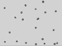
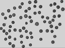


 (C: saturation capacity in 1000 electrons [ke], eNIR: enhanced NIR sensi- tivity, FR: frame rate in s− 1, ID: image diagonal in mm, QE: peak quantum effi ciency)


 π r 2
π r 2 π r|k|

 m=0n=0
 1 i
1 i


 √ 2π σ


 β = 2α , α = 1 + β − , 1 + 2β, β ∈ ] − 1/2, ∞ [


 = dΩ dA0 cos θ
  λ 5
λ 5


 sin(π Rk˜ ) 2R sin(π k˜ /2)
 √ 2R
√ 2R

 = 1 ˜ .
 Dx √ 2 ≈ 1.414
 D2x ±R 0.02 0.33 2.26 0.001 0.023 0.220 , 3 ln 3/π ≈ 1.024


 √ − 1 Imaginary unit