Multigrid Representations

Introduction

The scale spaces discussed so far have one signifi cant disadvantage. The use of the additional scale parameter adds a new dimension to the im- ages and thus leads to an explosion of the data storage requirements

5.3 Multigrid Representations                                                        137

 

and in turn the computational overhead for generating the scale space and for analyzing it. This diffi culty is the starting point for a new data structure for representing image data at diff erent scales, known as a multigrid representation.

The basic idea is quite simple. While the representation of fi ne scales requires the full resolution, coarser scales can be represented at lower resolution. This leads to a scale space with smaller and smaller images as the scale parameter increases. In the following two sections we will discuss the Gaussian pyramid (Section 5.3.2) and the Laplacian pyra- mid (Section 5.3.3) as effi cient discrete implementations of discrete scale spaces. While the Gaussian pyramid constitutes a standard scale space (Section 5.2.1), the Laplacian pyramid is a discrete version of a diff eren- tial scale space (Section 5.2.4). In this section, we only discuss the basics of multigrid representations. Optimal multigrid smoothing fi lters are elaborated in Section 11.6.

These pyramids are examples of multigrid data structures that have been introduced into digital image processing in the early 1980s and have led to a tremendous increase in speed of image processing algo- rithms in digital image processing since then.

 

Gaussian Pyramid

If we want to reduce the size of an image, we cannot just subsample the image by taking, for example, every second pixel in every second line. If we did so, we would disregard the sampling theorem (Section 9.2.3). For example, a structure which is sampled three times per wavelength in the original image would only be sampled one and a half times in the subsampled image and thus appear as an aliased pattern as we will discuss in Section 9.1. Consequently, we must ensure that all structures which are sampled less than four times per wavelength are suppressed by an appropriate smoothing fi lter to ensure a proper subsampled image. For the generation of the scale space, this means that size reduction must go hand in hand with appropriate smoothing.

Generally, the requirement for the smoothing fi lter can be formulated

as

rp

Bˆ ( k ˜ ) = 0  ∀ k˜ p ≥  1 ,                                              (5.46)

+

where r_p is the subsampling rate in the direction of the pth coordinate. The combined smoothing and size reduction can be expressed in a single operator by using the following notation to compute the q 1th

level of the Gaussian pyramid from the qth level:

G (q+1) = B_{↓ 2} G (q).                                              (5.47)

The number behind the ↓ in the index denotes the subsampling rate. The 0th level of the pyramid is the original image: G (0) = G.

138                                                                              5 Multiscale Representation

 

a                                                                    b

Figure 5.5: Gaussian pyramid: a schematic representation, the squares of the checkerboard corresponding to pixels; b example.

 

If we repeat the smoothing and subsampling operations iteratively, we obtain a series of images, which is called the Gaussian pyramid. From level to level, the resolution decreases by a factor of two; the size of the images decreases correspondingly. Consequently, we can think of the series of images as being arranged in the form of a pyramid as illustrated in Fig. 5.5.

The pyramid does not require much storage space. Generally, if we consider the formation of a pyramid from a W -dimensional image with a subsampling factor of two and M pixels in each coordinate direction, the total number of pixels is given by

2W

MW .1 +  1

1

+ 22W

W

Σ        2+

... < MW.        (5.48)      2W − 1

For a two-dimensional image, the whole pyramid needs only 1/3 more space than the original image for a three-dimensional image only 1/7 more. Likewise, the computation of the pyramid is equally eff ective. The same smoothing fi lter is applied to each level of the pyramid. Thus the computation of the whole pyramid only needs 4/3 and 8/7 times more operations than for the fi rst level of a two-dimensional and three- dimensional image, respectively.

The pyramid brings large scales into the range of local neighbor- hood operations with small kernels. Moreover, these operations are per- formed effi ciently. Once the pyramid has been computed, we can per-

5.3 Multigrid Representations                                                        139

 

form neighborhood operations on large scales in the upper levels of the pyramid — because of the smaller image sizes — much more effi ciently than for fi ner scales.

The Gaussian pyramid constitutes a series of lowpass-fi ltered images in which the cut-off wave numbers decrease by a factor of two (an octave) from level to level. Thus only the coarser details remain in the smaller images (Fig. 5.5). Only a few levels of the pyramid are necessary to span a wide range of wave numbers. From a 512 × 512 image we can usefully compute only a seven-level pyramid. The smallest image is then 8 × 8.

Laplacian Pyramid

From the Gaussian pyramid, another pyramid type can be derived, the Laplacian pyramid. This type of pyramid is the discrete counterpart to the diff erential scale space discussed in Section 5.2.4 and leads to a se- quence of bandpass-fi ltered images. In contrast to the Fourier transform, the Laplacian pyramid only leads to a coarse wave number decomposi- tion without a directional decomposition. All wave numbers, indepen- dently of their direction, within the range of about an octave (factor of two) are contained in one level of the pyramid.

Because of the coarse wave number resolution, we can preserve a good spatial resolution. Each level of the pyramid only contains match- ing scales which are sampled a few times (two to six) per wavelength. In this way, the Laplacian pyramid is an effi cient data structure well adapted to the limits of the product of wave number and spatial resolution set by the uncertainty relation (Theorem 7, p. 55).

↑

↑

The diff erentiation in scale direction in the continuous scale space is approximated by subtracting two levels of the Gaussian pyramid. In order to do so, fi rst the image at the coarser level must be expanded. This operation is performed by an expansion operator ₂. As with the reducing smoothing operator, the degree of expansion is denoted by the fi gure after the in the index.

The expansion is signifi cantly more diffi cult than the size reduction as the missing information must be interpolated. For a size increase of two in all directions, fi rst every second pixel in each row must be interpolated and then every second row. Interpolation is discussed in detail in Section 10.6. With the introduced notation, the generation of the pth level of the Laplacian pyramid can be written as:

L (p) = G (p)− ↑ ₂ G (p+1).                                           (5.49)

The Laplacian pyramid is an eff ective scheme for a bandpass decom- position of an image. The center wave number is halved from level to level. The last image of the Laplacian pyramid is a lowpass-fi ltered im- age containing only the coarsest structures.

140                                                                              5 Multiscale Representation

 

Figure 5.6: Construction of the Laplacian pyramid (right column) from the Gaussian pyramid (left column) by subtracting two consecutive planes of the Gaussian pyramid.

 

−

+

The Laplacian pyramid has the signifi cant advantage that the original image can be reconstructed quickly from the sequence of images in the Laplacian pyramid by recursively expanding the images and summing them up. The recursion is the inverse of the recursion in Eq. (5.49). In a Laplacian pyramid with p 1 levels, the level p (counting starts with zero! ) is the coarsest level of the Gaussian pyramid. Then the level p 1 of the Gaussian pyramid can be reconstructed by

G (p− 1) = L (p− 1)+ ↑ 2 G p                                                                  (5.50)

Note that this is just an inversion of the construction scheme for the Laplacian pyramid. This means that even if the interpolation algorithms required to expand the image contain errors, they aff ect only the Lapla- cian pyramid and not the reconstruction of the Gaussian pyramid from the Laplacian pyramid, as the same algorithm is used. The recursion in Eq. (5.50) is repeated with lower levels until level 0, i. e., the original image, is reached again. As illustrated in Fig. 5.6, fi ner and fi ner details become visible during the reconstruction process. Because of the pro-

5.3 Multigrid Representations                                                        141

 

X                                          y

1

2

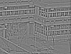
Figure 5.7: First three planes of a directiopyramidal decomposition of Fig. 5.3a: the rows show are planes 0, 1, and 2, the columns L, L _x, L _y according to Eqs. (5.52) and (5.53).

 

gressive reconstruction of details, the Laplacian pyramid has been used as a compact scheme for image compression. Nowadays, more effi cient schemes are available on the basis of wavelet transforms, but they oper- ate on principles very similar to those of the Laplacian pyramid.

 

⇐ Предыдущая24252627282930313233Следующая ⇒

Поделиться: