Color Coding of the 2-D Structure Tensor

⇐ ПредыдущаяСтр 60 из 85Следующая ⇒

In Section 13.2.3 we discussed a color representation of the orientation vector. The question is whether it is also possible to represent the struc- ture tensor adequately as a color image. A symmetric 2-D tensor has three independent pieces of information Eq. (13.14), which ﬁ t well to the three degrees of freedom available to represent color, for example luminance, hue, and saturation.

A color represention of the structure tensor requires only two slight modiﬁ cations as compared to the color representation for the orienta- tion vector. First, instead of the length of the orientation vector, the squared magnitude of the gradient is mapped onto the intensity. Sec- ond, the coherency measure Eq. (13.15) is used as the saturation. In the color representation for the orientation vector, the saturation is always one. The angle of the orientation vector is still represented as the hue.

In practice, a slight modiﬁ cation of this color representation is useful. The squared magnitude of the gradient shows variations too large to be displayed in the narrow dynamic range of a display screen with only 256

350 13 Simple Neighborhoods

luminance levels. Therefore, a suitable normalization is required. The basic idea of this normalization is to compare the squared magnitude of the gradient with the noise level. Once the gradient is well above the noise level it is regarded as a signiﬁ cant piece of information. This train of thoughts suggests the following normalization for the intensity I:

I = J 11 + J 22 , (13.16)

(J₁₁ + J₂₂) + γ σ 2

where σ _n is an estimate of the standard deviation of the noise level. This normalization provides a rapid transition of the luminance from one, when the magnitude of the gradient is larger than σ _n, to zero when the gradient is smaller than σ _n. The factor γ is used to optimize the display.

Implementation

The structure tensor (Section 13.3.1) or the inertia tensor (Section 13.3.7) can be computed straightforwardly as a combination of linear convolu- tion and nonlinear point operations. The partial derivatives in Eqs. (13.8) and (13.25) are approximated by discrete derivative operators. The inte- gration weighted with the window function is replaced by a convolution with a smoothing ﬁ lter which has the shape of the window function. If we denote the discrete partial derivative operator with respect to the co- ordinate p by the operator _p and the (isotropic) smoothing operator by, the local structure of a gray value image can be computed with the structure tensor operator

J_pq = B(D_p · D_q). (13.17)

D D

The equation is written in an operator notation. Pixelwise multiplication is denoted by · to distinguish it from successive application of convolu- tion operators. Equation Eq. (13.17) says, in words, that the _pq compo- nent of the tensor is computed by convolving the image independently with _p and _q, multiplying the two images pixelwise, and smoothing the resulting image with.

≥

These operators are valid in images of any dimension W 2. In a W - dimensional image, the structure tensor has W (W 1)/2 independent components, hence 3 in 2-D, 6 in 3-D, and 10 in 4-D images. These components are best stored in a multichannel image with W (W 1)/2 components.

The smoothing operations consume the largest number of opera- tions. Therefore, a fast implementation must, in the ﬁ rst place, apply a fast smoothing algorithm. A fast algorithm can be established based on the general observation that higher-order features always show a lower resolution than the features they are computed from. This means that

13.3 First-Order Tensor Representation† 351

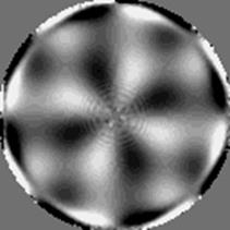
the structure tensor can be stored on a coarser grid and thus in a smaller image. A convenient and appropriate subsampling rate is to reduce the scale by a factor of two by storing only every second pixel in every second row.

These procedures lead us in a natural way to multigrid data struc- tures which are discussed in detail in Chapter 5. Multistep averaging is discussed in detail in Section 11.6.1.

Storing higher-order features on coarser scales has another signiﬁ - cant advantage. Any subsequent processing is sped up simply by the fact that many fewer pixels have to be processed. A linear scale reduc- tion by a factor of two results in a reduction in the number of pixels and the number of computations by a factor of 4 in two and 8 in three dimensions.

Figure 13.5 illustrates all steps to compute the structure tensor and derived quantities using the ring test pattern. This test pattern is par- ticularly suitable for orientation analysis since it contains all kinds of orientations and wave numbers in one image.

−

The accuracy of the orientation angle strongly depends on the imple- mentation of the derivative ﬁ lters. The straightforward implementation of the algorithm using the standard derivative ﬁ lter mask 1/2 [10 1] (Section 12.3.3) or the Sobel operator (Section 12.5.3) results in surpris-

ingly high errors (Fig. 13.6b), with a maximum error in the orientation angle of more than 7° at a wave number of k˜ 0.7. The error depends

on both the wave number and the orientation of the local structure. For orientation angles in the direction of axes and diagonals, the error van- ishes. The high error and the structure of the error map result from the transfer function of the derivative ﬁ lter. The transfer function shows signiﬁ cant deviation from the transfer function for an ideal derivative ﬁ lter for high wave numbers (Section 12.2). According to Eq. (13.12), the orientation angle depends on the ratio of derivatives. Along the axes, one of the derivatives is zero and, thus, no error occurs. Along the diagonals, the derivatives in the x and y directions are the same. Consequently, the error in both cancels in the ratio of the derivatives as well.

The error in the orientation angle can be signiﬁ cantly suppressed if better derivative ﬁ lters are used. Figure 13.6 shows the error in the orien- tation estimate using two examples of the optimized Sobel operator (Sec- tion 12.5.5) and the least-squares optimized operator (Section 12.3.5).

The little extra eﬀ ort in optimizing the derivative ﬁ lters thus pays oﬀ in an accurate orientation estimate. A residual angle error of less than 0.5° is suﬃ cient for almost all applications. The various derivative ﬁ lters discussed in Sections 12.3 and 12.5 give the freedom to balance computational eﬀ ort with accuracy.

An important property of any image processing algorithm is its ro- bustness. This term denotes the sensitivity of an algorithm against noise. Two questions are important. First, how large is the error of the esti-

352 13 Simple Neighborhoods

A b

C d

E f

G h

I j

Figure 13.5: Steps to compute the structure tensor: a original ring test pattern; b horizontal derivation D_x; c vertical derivation D_y; d – f averaged components for the structure tensor J₁₁ = B(D_x · D_x), J₂₂ = B(D_y · D_y), J₁₂ = B(D_x · D_y); g squared magnitude of gradient J₁₁ + J₂₂; h x component of orientation vector J₁₁ − J₂₂; i y component of orientation vector 2J₁₂; j orientation angle from [− π /2, π /2] mapped to a gray scale interval from [0, 255].

13.3 First-Order Tensor Representation† 353

A b

C d

= ±

Figure 13.6: Systematic errors for the orientation angle estimate using diﬀ erent derivative operators: a original ring test pattern with a maximum normalized wave number k˜ 0.7; error maps for b the Sobel operator (angle range 7◦ in 16 discrete steps), c the optimized Sobel operator, and d the least squares optimized operator (angle range ±0.7◦ in 16 discrete steps) with r = 3.

mated features in noisy images? To answer this question, the laws of statistics are used to study error propagation. In this context, noise makes the estimates only uncertain but not erroneous. The mean — if we make a suﬃ cient number of estimates — is still correct. However, a second question arises. In noisy images an operator can also give results that are biased, i. e., the mean can show a signiﬁ cant deviation from the correct value. In the worst case, an algorithm can even become unstable and deliver meaningless results.

354 13 Simple Neighborhoods

A b

C d

1 1

0.98 0.8

0.96 0.6

0.94 0.4

0.92

0.9 0 20 40 60 80 100 120 x




		5.0
		1.5

0.8

0.6

0.4

0.2

0.8

0.6

0.4

0 20 40 60 80 100 120x

0.2

-2 -1 0 1 angle[°] 2

0.2

0 -20 -10 0 10 angle[°]20

Figure 13.7: Orientation analysis with a noisy ring test pattern using the op- timized Sobel operator: ring pattern with amplitude 50, standard deviation of normal distributed noise a 15, and b 50; c and d radial cross section of the co- herency measure for standard deviations of the noise level of 1.5 and 5, 15 and 50, respectively; e and f histograms of angle error for the same conditions.

Figure 13.7 demonstrates that the estimate of orientation is also a re- markably robust algorithm. Even with a low signal-to-noise ratio, the ori- entation estimate is still correct if a suitable derivative operator is used. With increasing noise level, the coherency (Section 13.3.4) decreases and the statistical error of the orientation angle estimate increases (Fig. 13.7).

13.3 First-Order Tensor Representation† 355

13.3.7 The Inertia Tensor‡

In this section, we discuss an alternative approach to describe the local structure in images. As a starting point, we consider what an ideally oriented gray value structure (Eq. (13.1)) looks like in the wave number domain. We can compute the Fourier transform of Eq. (13.1) more readily if we rotate the x₁ axis in the direction of n ¯. Then the gray value function is constant in the x₂ direction. Consequently, the Fourier transform reduces to a δ line in the direction of n ¯ (± R5).

It seems promising to determine local orientation in the Fourier domain, as all we have to compute is the orientation of the line on which the spectral densities are non-zero. Bigü n and Granlund [8] devised the following procedure:

• Use a window function to select a small local neighborhood from an image.

•

Fourier transform the windowed image. The smaller the selected window, the more blurred the spectrum will be (uncertainty relation, Theorem 7, p. 55). This means that even with an ideal local orientation we will obtain a rather band-shaped distribution of the spectral energy.

•

Determine local orientation by ﬁ tting a straight line to the spectral density distribution. This yields the angle of the local orientation from the slope of the line.

The critical step of this procedure is ﬁ tting a straight line to the spectral densi- ties in the Fourier domain. We cannot solve this problem exactly as it is gener- ally overdetermined, but only minimize the measure of error. A standard error measure is the square of the magnitude of the vector (L₂ norm; see Eq. (2.74) in Section 2.4.1). When ﬁ tting a straight line, we minimize the sum of the squares of the distances of the data points to the line:

∞

∫ d2( k, n ¯ )|gˆ ( k )|2d^W k → minimum. (13.18)

− ∞

| |

The distance function is abbreviated using d( k, n ¯ ). The integral runs over the whole wave number space; the wave numbers are weighted with the spectral density gˆ ( k ) 2. Equation (13.18) is not restricted to two dimensions, but is gen- erally valid for local orientation or linear symmetry in a W -dimensional space.

The distance vector d can be inferred from Fig. 13.8 to be

d = k − ( k ^T n ¯ ) n ¯. (13.19)

The square of the distance is then given by

| d |2 = | k − ( k ^T n ¯ ) n ¯ |2 = | k |2 − ( k ^T n ¯ )2. (13.20)

In order to express the distance more clearly as a function of the vector n ¯, we rewrite it in the following manner:

| d |2 = n ¯ ^T ( I ( k ^T k ) − ( kk ^T )) n ¯, (13.21)

where I is the unit diagonal matrix. Substituting this expression into Eq. (13.18) we obtain

n ¯ ^T J ' n ¯ → minimum, (13.22)

356 13 Simple Neighborhoods

Figure 13.8: Distance of a point in the wave number space from the line in the direction of the unit vector n ¯.

where J ' is a symmetric tensor with the diagonal elements

. ∫ ' ˆ J = k |g(k)| d k (13.23)pp

∞

2 2 W

q≠ p− ∞

and the oﬀ -diagonal elements

∞

J_p' q =− ∫ k_pk_q|gˆ ( k )|2d^W k, p ≠ q. (13.24)

− ∞

| |

The tensor J ' is analogous to a well-known physical quantity, the inertia tensor. If we replace the wave number coordinates by space coordinates and the spectral density gˆ ( k ) 2 by the speciﬁ c density ρ, Eqs. (13.18) and (13.22) constitute the equation to compute the inertia of a rotary body rotating around the n ¯ axis.

With this analogy, we can reformulate the problem of determining local ori- entation. We must ﬁ nd the axis about which the rotary body, formed from the spectral density in Fourier space, rotates with minimum inertia. This body might have diﬀ erent shapes. We can relate its shape to the diﬀ erent solutions we get for the eigenvalues of the inertia tensor and thus for the solution of the local orientation problem (Table 13.3).

We derived the inertia tensor approach in the Fourier domain. Now we will show how to compute the coeﬃ cients of the inertia tensor in the space domain.

The integrals in Eqs. (13.23) and (13.24) contain terms of the form

k2 |gˆ ( k )|2 = |ik_qgˆ ( k )|2

and

k_pk_q|gˆ ( k )|2 = ik_pgˆ ( k )[ik_qgˆ ( k )]∗.

Integrals over these terms are inner or scalar products of the functions ik_pgˆ ( k ). Because the inner product is preserved under the Fourier transform ( R4), we can compute the corresponding integrals in the spatial domain as well. Multipli- cation of gˆ ( k ) with ik_p in the wave number domain corresponds to performing

13.3 First-Order Tensor Representation† 357

Table 13.3: Eigenvalue classiﬁ cation of the structure tensor in 3-D (volumetric) images.

Condition Explanation

Ideal local orientation The rotary body is a line. For a rotation around

this line, the inertia vanishes. Consequently, the eigenvector to the eigenvalue zero coin- cides with the direction of the line. The other eigenvector is orthogonal to the line, and the corresponding eigenvalue is unequal to zero and gives the rotation axis for maximum iner- tia.

Isotropic gray value structure

In this case, the rotary body is a kind of ﬂ at isotropic disk. A preferred direction does not exist. Both eigenvalues are equal and the in- ertia is the same for rotations around all axes. We cannot ﬁ nd a minimum.

Constant gray values The rotary body degenerates to a point at the

origin of the wave number space. The inertia is zero for rotation around any axis. Therefore both eigenvalues vanish.

the ﬁ rst spatial derivative in the direction of x_p in the space domain:

J_p' p( x ) =

. ∫ w( x − x ')

. Σ ∂ g

dW x'

∂ x

∞

q≠ p − ∞ q

∞

(13.25)

pq ∂ x_p ∂ x_q

J' ( x ) = − ∫ w( x − x ') ∂ g ∂ g d^W x'.

− ∞

In Eq. (13.25), we already included the weighting with the window function w

to select a local neighborhood.

The structure tensor discussed in Section 13.3.1 Eq. (13.8) and the inertia tensor are closely related:

J ' = trace( J ) I − J. (13.26)

From this relationship it is evident that both matrices have the same set of eigenvectors. The eigenvalues λ _p are related by

n n

λ _p =. λ _q − λ 'p, λ 'p =. λ _q − λ _p. (13.27)

q=1 q=1

Consequently, we can perform the eigenvalue analysis with any of the two ma- trices. For the inertia tensor, the direction of local orientation is given by the minimum eigenvalue, but for the structure tensor it is given by the maximum eigenvalue.

358 13 Simple Neighborhoods

13.3.8 Further Equivalent Approaches‡

In their paper on analyzing oriented patterns, Kass and Witkin [90] chose — at ﬁ rst glance — a completely diﬀ erent method. Yet it turns out to be equivalent to the tensor method, as will be shown in the following. They started with the idea of using directional derivative ﬁ lters by diﬀ erentiating a diﬀ erence of Gaussian ﬁ lter (DoG, Section 12.5.6) (written in operator notation)

D (B − B )_y ₁ ₂

R_y

R(Θ ) = [cos Θ sin Θ ] Σ Dx(B1 − B2) Σ = [cos Θ sin Θ ] Σ Rx Σ ,

B B

where ₁ and ₂ denote two Gaussian smoothing masks with diﬀ erent vari- ances. The direction in which this directional derivative is maximal in a mean square sense gives the orientation normal to lines of constant gray values. This approach results in the following expression for the variance of the directional derivative:

V (Θ ) = B(R(Θ ) · R(Θ )). (13.28)

The directional derivative is squared and then smoothed by a binomial ﬁ lter. This equation can also be interpreted as the inertia of an object as a function of the angle. The corresponding inertia tensor has the form

Σ Σ . (13.29)

B(R_y · R_y) − B(R_x · R_y)

− B(R_x · R_y) B(R_x · R_x)

Thus Kass and Witkin’s approach is identical to the general inertia tensor method discussed in Section 13.3.7. They just used a special type of derivative ﬁ lter.

Without being aware of either Bigü n and Granlund [8] earlier or Knutsson [99] contemporary work, Rao and Schunck [147] and Rao [146] proposed the same structure tensor (denoting it as the moment tensor) as that we discussed in Section 13.3.1.

13.4 Local Wave Number and Phase‡

13.4.1 Phase‡

So far in this chapter we have discussed in detail the analysis of simple neighbor- hoods with respect to their orientation. In this section we proceed with another elementary property of simple neighborhoods. In Chapter 5 we stressed the importance of the scale for image processing. Thus we must not only ask in which directions the gray values change. We must also ask how fast the gray values change. This question leads us to the concept of the local wave number.

The key to determining the local wave number is the phase of the signal. As an introduction we discuss a simple example and consider the one-dimensional periodic signal

g(x) = g₀ cos(kx). (13.30)

The argument of the cosine function is known as the phase of the periodic signal:

φ (x) = kx. (13.31)

13.4 Local Wave Number and Phase‡ 359

Figure 13.9: Application of the Hilbert ﬁ lter to the ring test pattern: upper left quadrant: in the horizontal direction; lower right quadrant: in the vertical direc- tion.

The equation shows that the phase is a linear function of the position and the wave number. Thus we obtain the wave number of the periodic signal by com- puting the ﬁ rst-order spatial derivative of the phase signal

∂ φ (x)

∂ x = k. (13.32)

These simple considerations re-emphasize the signiﬁ cant role of the phase in image processing that we discussed already in Section 2.3.6. We will discuss two related approaches for determining the phase of a signal, the Hilbert transform (Section 13.4.2) and the quadrature ﬁ lter (Section 13.4.5) before we introduce eﬃ cient techniques to compute the local wave number from phase gradients.

13.4.2 Hilbert Transform and Hilbert Filter‡

= =

In order to explain the principle of computing the phase of a signal, we take again the example of the simple periodic signal from the previous section. We suppose that an operator is available to delay the signal by a phase of 90°. This operator would convert the g(x) g₀ cos(kx) signal into a g'(x)

−

g₀ sin(kx) signal as illustrated in Fig. 13.9. Using both signals, the phase of g(x) can be computed by

= . Σ

φ (g(x)) arctan − g'(x) . (13.33)

g(x)

360 13 Simple Neighborhoods

As only the ratio of g'(x) and g(x) goes into Eq. (13.33), the phase is indeed independent of amplitude. If we take the signs of the two functions g'(x) and g(x) into account, the phase can be computed over the full range of 360°.

Thus all we need to determine the phase of a signal is a linear operator that shifts the phase of a signal by 90°. Such an operator is known as the Hilbert ﬁ lter H or Hilbert operator H and has the transfer function

hˆ (k) =

  

i k> 0

0 k = 0

. (13.34)



 − i k< 0

− −

The magnitude of the transfer function is one as the amplitude remains un- changed. As the Hilbert ﬁ lter has a purely imaginary transfer function, it must be of odd symmetry to generate a real-valued signal. Therefore positive wave numbers are shifted by 90° (π /2) and negative wave numbers by 90° ( π /2). A special situation is given for the wave number zero where the transfer function is also zero. This exception can be illustrated as follows. A signal with wave number zero is a constant. It can be regarded as a cosine function with inﬁ - nite wave number sampled at the phase zero. Consequently, the Hilbert ﬁ ltered signal is the corresponding sine function at phase zero, that is, zero.

Because of the discontinuity of the transfer function of the Hilbert ﬁ lter at the origin, its point spread function is of inﬁ nite extent

=−

h(x) 1

π x

. (13.35)

The convolution with Eq. (13.35) can be written as

∞

g_h(x) = 1 ∫ g(x') dx'. (13.36)

π − ∞ x' − x

This integral transform is known as the Hilbert transform [116].

Because the convolution mask of the Hilbert ﬁ lter is inﬁ nite, it is impossible to design an exact discrete Hilbert ﬁ lter for arbitrary signals. This is only possible if we restrict the class of signals to which it is applied. Thus the following approach is taken to design an eﬀ ective implementation of a Hilbert ﬁ lter.

First, the ﬁ lter should precisely shift the phase by π /2. This requirement comes from the fact that we cannot aﬀ ord an error in the phase because it includes the position information. A wave-number dependent phase shift would cause wave-number dependent errors. This requirement is met by any convolution kernel of odd symmetry.

Second, requirements for a magnitude of one can be relaxed if the Hilbert ﬁ lter is applied to a bandpassed signal, e. g., the Laplace pyramid. Then, the Hilbert ﬁ lter must only show a magnitude of one in the passband range of the bandpass ﬁ lter used. This approach avoids the discontinuities in the transfer function at the wave number zero and thus results in ﬁ nite-sized convolution kernels.

Optimized Hilbert ﬁ lters are generated with the same least-squares techniques used above for interpolation ﬁ lters (Section 10.6.6) and ﬁ rst-order derivative ﬁ lters (Section 12.3.5).

13.4 Local Wave Number and Phase‡ 361

1 4

0.8 5

0.6 2

0.4

0.2

1.04

1.02

0.98

0.96

0 0 0.1 0.2 0.3 0.4

~ 0.5

0 0.1 0.2 0.3 0.4 ~

0.5

Figure 13.10: a Transfer functions of a family of least-squares optimized Hilbert operators according to Eq. (13.37) for the four ﬁ lter coeﬃ cients R 2, 3, 4, 5. b sector of a to better show the deviations from an ideal Hilbert ﬁ lter. As the ﬁ lters are symmetric around k˜ = 0.5 only a wave number range from 0–0.5 is shown.

Because of the odd symmetry of the Hilbert ﬁ lter, the following formulation is used

. . Σ

hˆ (k˜ ) = 2i h_v sin (2v − 1)π k˜ . (13.37)

v=1

Note that we have only used sine functions with odd wave numbers. This causes the transfer function also to become symmetric around k˜ 1/2 and leads to a ﬁ lter mask with alternating zeros

[h_R, 0, ···, h₂, 0, h₁, 0, –h₁, 0, –h₂, ···, 0, –h_R]. (13.38)

− −

The mask has 4R 1 coeﬃ cients, 2R 1 of which are zero. Figure 13.10 shows the transfer functions optimized with the least squares technique for R = 2, 3, 4, 5. The ﬁ lter with R = 4 (a mask with 15 coeﬃ cients)

h = {0.6208, 0.1683, 0.0630, 0.0191}, (13.39)

for instance, has an amplitude error of only slightly larger than 1.0 % in the wave number range [0.16, 0.84] and by design no phase error. The convolution with this mask requires 4 multiplications and 7 additions/subtractions.

13.4.3 Analytic Signal‡

A real-valued signal and its Hilbert transform can be combined into a complex- valued signal by

g_a = g − ig_h. (13.40)

This complex-valued signal is denoted as the analytic function or analytic signal. According to Eq. (13.40) the analytic ﬁ lter has the point spread function

= +

a(x) 1 i

π x

(13.41)

362 13 Simple Neighborhoods

and the transfer function

aˆ (k) =

2 k> 0

  

1 k = 0

  0 k< 0

. (13.42)

Thus all negative wave numbers are suppressed. Although the transfer function of the analytic ﬁ lter is real, it results in a complex signal because it is asymmet- ric. For a real signal no information is lost by suppressing the negative wave numbers. They can be reconstructed as the Fourier transform of a real signal is Hermitian (Section 2.3.5). The analytic signal can be regarded as just another representation of a real signal with two important properties. The magnitude of the analytic signal gives the local amplitude

|A|2 = I ·I +H ·H. (13.43)

and the argument the local phase

arg(A) = arctan. − H Σ , (13.44) using A and H for the analytic and Hilbert operators, respectively.

The original signal and its Hilbert transform can be obtained from the analytic signal using Eq. (13.40) by

g(x) = (g_a(x) + g_a∗ (x))/2

g_h(x) = i(g_a(x) − g_a∗ (x))/2.

(13.45)

The concept of the analytic signal also makes it easy to extend the ideas of local phase into multiple dimensions. The transfer function of the analytic operator uses only the positive wave numbers, i. e., only half of the Fourier space. If we extend this partitioning to multiple dimensions, we have more than one choice to partition the Fourier space into two half spaces. Instead of the wave number, we can take the scalar product between the wave number vector k and any unit vector n ¯ and suppress the half space for which the scalar product k n ¯ is negative:

aˆ ( k ) =

1 k n ¯ = 0

   2 k n ¯ > 0

  0 k n ¯ < 0

. (13.46)

The unit vector n ¯ gives the direction in which the Hilbert ﬁ lter is to be applied. The deﬁ nition Eq. (13.46) of the transfer function of the analytic signal implies that the Hilbert operator can only be applied to directionally ﬁ ltered signals. This results from the following considerations. For one-dimensional signals we have seen that a discrete Hilbert ﬁ lter does not work well for small wave numbers (Fig. 13.10). In multiple dimensions this means that a Hilbert ﬁ lter does not work well if k ˜ n ¯ 1. Thus no wave numbers near an orthogonal to the direction of the Hilbert ﬁ lter may exist, in order to avoid errors.

This fact makes the application of Hilbert ﬁ lters and thus the determination of the local phase in higher-dimensional signals signiﬁ cantly more complex. It is not suﬃ cient to use bandpass ﬁ ltered images, e. g., a Laplace pyramid (Sec- tion 5.3.3). In addition, the bandpass ﬁ ltered images must be further decom- posed into directional components. At least as many directional components as the dimensionality of the space are required.

13.4 Local Wave Number and Phase‡ 363

13.4.4 Monogenic Signal‡

The extension of the Hilbert transform from a 1-Dsignal to higher-dimensional signals is not satisfactory because it can only be applied to directionally ﬁ ltered signals. For wave numbers close to the separation plane, the Hilbert transform does not work. What is really required is an isotropic extension of the Hilbert transform. It is obvious that no scalar-valued transform for a multidimensional signal can be both isotropic and of odd symmetry.

A vector-valued extension of the analytic signal meets both requirements. It is known as the monogenic signal and was introduced to image processing by Felsberg and Sommer [38]. The monogenic signal is constructed from the origi- nal signal and its Riesz transform. The transfer function of the Riesz transform is given by

h ˆ ( k ) i k . (13.47)

| k |

The magnitude of the vector h is one for all values of k. The Riesz transform is thus isotropic. It is also of odd symmetry because

h ˆ (− k ) = − h ˆ ( k ). (13.48)

The Riesz transform can be applied to a signal of any dimension. For a 1-D signal it reduces to the Hilbert transform.

For a 2-D signal the transfer function of the Riesz transform can be written using polar coordinates as

h ˆ ( k ) = i  k co s θ , k si n θ 

. (13.49)

|k| |k|

The convolution mask or PSF of the Riesz transform is given by

=−

h ( x ) x

2π | x |3

. (13.50)

The original signal and the signal convolved by the Riesz transform can be combined for a 2-Dsignal to the 3-Dmonogenic signal as

g _m( x ) = Σ g, h₁ ∗ g, h₂ ∗ gΣ . (13.51)

The local amplitude of the monogenic signal is given as the norm of the vector of the monogenic signal as in the case of the analytic signal (Eq. (13.43)):

g_m

. . = g2 + (h₁ ∗ g)2 + (h₂ ∗ g)2. (13.52)

For an intrinsically 1-D signal, it can be proven that the local phase φ and the local orientation θ are

and

tan φ =

1/2

Σ Σ 2 2(h ∗ g) + (h ∗ g)

1 2

(13.53)

tan θ h 2 ∗ g . (13.54)

h₁ ∗ g

We can thus conclude that the monogenic signal combines an estimate of local orientation (Section 13.2) and local phase (Section 13.4.1).

364 13 Simple Neighborhoods

13.4.5 Quadrature Filters‡

Quadrature ﬁ lters are an alternative approach to getting a pair of signals that diﬀ er only by a phase shift of 90° (π /2). It is easiest to introduce the complex form of the quadrature ﬁ lters. Essentially, the transfer function of a quadrature ﬁ lter is also zero for k n ¯ < 0, like the transfer function of the analytic ﬁ lter. However, the magnitude of the transfer function is not one but can be any arbitrary real-valued function h( k ):

.q(k) =

ˆ 2h( k ) k n ¯ > 0

0 otherwise.

(13.55)

The quadrature ﬁ lter thus also transforms a real-valued signal into an analyt- ical signal. In contrast to the analytical operator, a wave number weighting is applied. From the complex form of the quadrature ﬁ lter, we can derive the real quadrature ﬁ lter pair by observing that they are the part of Eq. (13.55) with even and odd symmetry. Thus

gˆ ₊( k ) = (qˆ ( k ) + qˆ (− k ))/2,

gˆ ₋( k ) = (qˆ ( k ) − qˆ (− k ))/2.

(13.56)

The even and odd part of the quadrature ﬁ lter pair show a phase shift of 90° and can thus can also be used to compute the local phase.

otherwise. (13.57)

The best-known quadrature ﬁ lter pair is the Gabor ﬁ lter. A Gabor ﬁ lter is a bandpass ﬁ lter that selects a certain wavelength range around the center wave- length k ₀ using the Gauss function. The complex transfer function of the Gabor ﬁ lter is

g( k )

. exp.| k − k ₀|2σ 2/2Σ kk ₀ > 0

If | k ₀|σ _x > 3, Eq. (13.57) reduces to

gˆ ( k ) = exp.− | k − k ₀)|2σ 2/2Σ . (13.58)

Using the relations in Eq. (13.56), the transfer function for the even and odd component are given by

gˆ ₊( k ) =

Σ exp.− | k − k ₀|2σ 2/2Σ + exp.− | k + k ₀|2σ 2/2Σ Σ ,

2 x x

(13.59)

gˆ ₋( k ) =

Σ exp.− | k − k ₀|2σ 2/2Σ − exp.− | k + k ₀|2σ 2/2Σ Σ .

The point spread function of these ﬁ lters can be computed easily with the shift theorem (Theorem 3, p. 52, ± R4):

g₊( x ) =

cos( k ₀ x ) exp.

x 2

Σ | |

− 2σ 2,

(13.60)

g₋( x ) =

i sin( k ₀ x ) exp.

x 2

Σ | |

− 2σ 2,

13.4 Local Wave Number and Phase‡ 365

or combined into a complex ﬁ lter mask:

g( x ) =

exp(i k ₀ x ) exp.

x 2

Σ | |

− 2σ 2 . (13.61)

Gabor ﬁ lters are useful for bandpass-ﬁ ltering images and performing image analysis in the space/wave number domain. Figure 13.11 illustrates an appli- cation [Riemer, 1991; Riemer et al., 1991]. An image with short wind-generated water surface waves is decomposed by a set of Gabor ﬁ lters. The center wave- length k ₀ was set in the x direction, parallel to the wind direction. The ﬁ lters had the center wavelength in octave distances at 1.2, 2.4, and 4.8 cm wavelengths. The bandwidth was set proportional to the center wave number.

The left column of images in Fig. 13.11 shows the ﬁ ltering with the even Ga- bor ﬁ lter, the right column the local amplitude, which is directly related to the energy of the waves. The ﬁ ltered images show that waves with diﬀ erent wave- length are partly coupled. In areas where the larger waves have large ampli- tudes, also the small-scale waves (capillary waves) have large amplitudes. The energy of waves is not equally distributed over the water surface.

An extension of this analysis to image sequences gives a direct insight into the nonlinear wave-wave interaction processes. Figure 13.12 shows the temporal evolution of one row of images from Fig. 13.11. As we will discuss in detail in Section 14.2.4, the slope of the structures in these space-time images towards the time axis is directly proportional to the speed of the moving objects.

It can be observed nicely that the small waves are modulated by the large waves and that the group velocity (speed of the wave energy) of the small waves is slower than the phase speed for the capillary waves.

13.4.6 Local Wave Number Determination‡

In order to determine the local wave number, we just need to compute the ﬁ rst spatial derivative of the phase signal (Section 13.4.1, Eq. (13.32)). This derivative has to be applied in the same direction as the Hilbert or quadrature ﬁ lter has been applied. The phase is given by either

. Σ =

φ ( x ) arctan − g h ( x ) (13.62)

g( x )

. Σ =

φ ( x ) arctan − g + ( x ) , (13.63)

g₋( x )

where g₊ and g₋ denote the signals ﬁ ltered with the even and odd part of the quadrature ﬁ lter.

Direct computation of the partial derivatives from Eqs. (13.62) and (13.63) is not advisable, however, because of the inherent discontinuities in the phase signal. A phase computed with the inverse tangent restricts the phase to the main interval [− π, π [ and thus leads inevitably to a wrapping of the phase signal from π to − π with the corresponding discontinuities.

366 13 Simple Neighborhoods

B c

D e

F g

Figure 13.11: Analysis of an image ( a, 40 cm 30 cm) from wind-generated water surface waves. The intensity is proportional to the along-wind component of the slope of the waves. The even part ( b, d, f ) and squared magnitude (energy, c, e, g ) of the Gabor-ﬁ ltered images with center wavelength at 48, 24, and 12 mm, respectively.

13.4 Local Wave Number and Phase‡ 367

A b c

D e f

Figure 13.12: Analysis of a 5 s long space-time slice in wind direction of an image sequence from short wind-generated water surface waves. The time axis is vertically oriented. Even part ( a – c ) and squared magnitude (energy, d – f ) of the Gabor-ﬁ ltered images with center wavelength at 48, 24, and 12 mm, respectively.

As pointed out by Fleet [42], this problem can be avoided by computing the phase gradient directly from the gradients of q₊( x ) and q₋( x ). The result is

=_p

k ∂ φ ( x )

∂ x_p

∂

= ∂ xp arctan(− q₊( x )/q₋( x ))

(13.64)

= 1 . ∂ q ₊ ( x ) q

( x ) − ∂ q − ( x ) q

( x )Σ .

−

q² ( x ) + q² ( x ) ∂ xp −

∂ x_p ⁺

This formulation of the phase gradient also eliminates the need for using trigono- metric functions to compute the phase signal and is, therefore, signiﬁ cantly faster.

368 13 Simple Neighborhoods

13.5 Tensor Representation by Quadrature Filter Sets‡

13.5.1 Principle‡

Quadrature ﬁ lters provide another way to analyze simple neighborhoods and to determine both the local orientation and the local wave number. Historically, this was the ﬁ rst technique for local structure analysis, pioneered by the work of Granlund [56]. The inertia and structure tensor techniques actually appeared later in the literature [8, 90, 146, 147].

The basic idea of the quadrature ﬁ lter set technique is to extract structures in a certain wave number and direction range. In order to determine local orien- tation, we must apply a whole set of directional ﬁ lters, with each ﬁ lter being sensitive to structures of diﬀ erent orientation. We then compare the ﬁ lter re- sponses and obtain a maximum ﬁ lter response from the directional ﬁ lter whose direction coincides best with that of local orientation. Similarly, the quadrature ﬁ lter set for diﬀ erent wave number ranges can be set up to determine the local wave number.

If we get a clear maximum in one of the ﬁ lters but only little response in the others, the local neighborhood contains a locally oriented pattern. If the diﬀ er- ent ﬁ lters give comparable responses, the neighborhood contains a distribution of oriented patterns.

So far, the concept seems to be straightforward, but a number of tricky problems needs to be solved. Which properties have to be met by the directional ﬁ lters in order to ensure an exact determination of local orientation, if at all possible? For computational eﬃ ciency, we need to use a minimal number of ﬁ lters to interpolate the angle of the local orientation. What is this minimal number?

The concepts introduced in this section are based on the work of Granlund [56], Knutsson [98], and Knutsson et al. [100], later summarized in a monograph by Granlund and Knutsson [57]. While the quadrature ﬁ lter set techniques have been formulated by these authors for multiple dimensions, we will discuss here only the two-dimensional case.

We ﬁ rst discuss the design of quadrature ﬁ lters that are suitable for the de- tection of both local orientation and local wave number. This leads to polar separable quadrature ﬁ lters (Section 13.5.2). In a second step, we show how the orientation vector deﬁ ned in Section 13.3.3 can be constructed by simple vector addition of the quadrature ﬁ lter responses (Section 13.5.3). Likewise, in Section 13.5.4 we study the computation of the local wave number. Finally, Section 13.5.5 closes the circle by showing that the structure tensor can also be computed by a set of quadrature ﬁ lters. Thus the tensor methods discussed in the ﬁ rst part of this chapter (Section 13.3) and the quadrature ﬁ lter set tech- nique diﬀ er only in some subtle points but otherwise give identical results.

13.5.2 Polar Separable Quadrature Filters‡

For an appropriate set of directional ﬁ lters, each ﬁ lter should be a rotated copy of the others. This requirement implies that the transfer function of the ﬁ lters can be separated into an angular part d(φ ) and a wave number part r(k). Such a ﬁ lter is called polar separable and may be conveniently expressed in polar

13.5 Tensor Representation by Quadrature Filter Sets‡ 369

coordinates

qˆ (k, φ ) = rˆ (k)dˆ (φ ), (13.65)

where k =  k2 + k2 and φ = arctan(k₂/k₁) are the magnitude and argument of

the wave number, respectively. For a set of directional ﬁ lters, only the angular part of the transfer function is of importance, while the radial part must be the same for each ﬁ lter but can be of arbitrary shape. The converse is true for a ﬁ lter set to determine the local wave number.

Knutsson [98] suggested the following base quadrature ﬁ lter

rˆ (k) =

exp Σ −

(ln k − ln k₀)2 (B/2)2 ln 2

(13.66)

dˆ (φ ) =

cos2l(φ − φ _k) |φ − φ _k| < π /2

0 otherwise.

In this equation, the complex notation for quadrature ﬁ lters is used (Section 13.4.5). The ﬁ lter is directed into the angle φ _k. The unit vector in this direction is d ¯ k = [cos φ _k, sin φ _k].

| − |= =

The ﬁ lter is continuous, since the cosine function is zero in the partition plane for the two half spaces ( φ φ _k π /2 or d ¯ k k 0). Using the unit vector d ¯ k in the direction of the ﬁ lter, the angular part of the ﬁ lter can also be written as:

dˆ ( k ) =

( k d ¯ k)2l ( k d ¯ k)> 0

(13.67)

0 otherwise.

The constant k₀ in Eq. (13.66) denotes the peak wave number. The constant B determines the half-width of the wave number in number of octaves and l the angular resolution of the ﬁ lter. In a logarithmic wave number scale, the ﬁ lter has the shape of a Gaussian function. Therefore the radial part has a lognormal shape.

For the real even and the imaginary odd ﬁ lter of the quadrature ﬁ lter pair, the radial part is the same and only the angular part diﬀ ers:

dˆ (φ ) = cos2l(φ − φ )

+ k (13.68)

−

dˆ (φ ) = i cos2l(φ − φ ) sign(cos(φ − φ )).

Figure 13.13 shows the radial and angular part of the transfer function for dif- ferent k₀ and φ _k. A set of directional ﬁ lters is obtained by a suitable choice of diﬀ erent φ _k:

φ k = π k

k = 0, 1, ···, K − 1. (13.69)

Knutsson used four ﬁ lters with 45° increments in the directions 22.5°, 67.5°, 112.5°, and 157.5°. These directions have the advantage that only one ﬁ lter kernel has to be designed. The kernels for the ﬁ lter in the other directions are obtained by mirroring the kernels at the axes and diagonals.

These ﬁ lters were designed in the wave number space. The ﬁ lter coeﬃ cients are obtained by inverse Fourier transformation. If we choose a reasonably small ﬁ lter mask, we will cut oﬀ a number of non-zero ﬁ lter coeﬃ cients. This causes deviations from the ideal transfer function.

370 13 Simple Neighborhoods

0.8

0.6 0.6

0.4 0.4

0.2

0 0.5 1 1.5 2 2.5 f 3

= =

Figure 13.13: a Radial and b angular part of quadrature ﬁ lter according to Eq. (13.66) with l 1 and B 2 in diﬀ erent directions and with diﬀ erent peak wave numbers.

Figure 13.14: Computation of local orientation by vector addition of the four ﬁ lter responses. An example is shown where the neighborhood is isotropic con- cerning orientation: all four ﬁ lter responses are equal. The angles of the vectors are equal to the ﬁ lter directions in a and double the ﬁ lter directions in b .

Therefore, Knutsson modiﬁ ed the ﬁ lter kernel coeﬃ cient using an optimization procedure in such a way that it approaches the ideal transfer function as closely as possible. It turned out that at least a 15 15 ﬁ lter mask is necessary to get a good approximation of the anticipated transfer function.

13.5.3 Determination of the Orientation Vector‡

The local orientation can be computed from the responses of the four quadra- ture ﬁ lters by vector addition. The idea of the approach is simple. We assign to the individual directional ﬁ lters an orientation vector. The magnitude of the vector corresponds to the response of the quadrature ﬁ lter. The direction of the vector is given by the double angle of the ﬁ lter direction (Section 13.3.3). In this representation each ﬁ lter response shows how well the orientation of the pattern is directed in the direction of the ﬁ lter. An estimate of the orientation vector is then given as the vector sum of the ﬁ lter responses.

13.5 Tensor Representation by Quadrature Filter Sets‡ 371

Using a represention with complex numbers for the orientation vector, we can write the ﬁ lter response for the ﬁ lter in φ _k direction as

Q_φk = |Q| exp(2iφ _k). (13.70)

Then the orientation vector as the vector sum of the ﬁ lter responses can be written as

K− 1

O= Q_φk. (13.71)

k=0

Figure 13.14 illustrates why an angle doubling is necessary for the vector addi- tion to obtain the orientation vector. An example is taken where the responses from all four ﬁ lters are equal. In this case the neighborhood contains structures in all directions. Consequently, we observe no local orientation and the vector sum of all ﬁ lter responses vanishes. This happens if we double the orientation angle (Fig. 13.14b), but not if we omit this step (Fig. 13.14a).

After these more qualitative considerations, we will prove that we can compute the local orientation exactly when the local neighborhood is ideally oriented in an arbitrary direction φ ₀. As a result, we will also learn the least number of ﬁ lters we need. We can simplify the computations by only considering the angular terms, as the ﬁ lter responses show the same wave number dependence. The quick reader can skip this proof.

Using Eq. (13.70), Eq. (13.66), and Eq. (13.69) we can write the angular part of the ﬁ lter response of the kth ﬁ lter as

dˆ k(φ ₀) = exp (2π ik/K) cos²^l(φ ₀ − π k/K).

The cosine function is decomposed into the sum of two complex exponentials:

22l

dˆ k(φ ₀) = 1

exp (2π ik/K) [exp (i(φ ₀ − π k/K)) + exp (− i(φ ₀ − π k/K))]^2l

1 ²

.2lΣ

= 22l exp (2π ik/K) j

j=0

exp.ij(φ ₀ − π k/K)Σ exp.− i(2l − j)(φ ₀ − π k/K)Σ

1 2l

.2lΣ

= 22l j.=0 j

exp.i(j − l)2φ ₀Σ exp.2π i(1 + l − j)(k/K)Σ .

Now we sum up the vectors of all the K directional ﬁ lters:

k=0

22l j=0

k=0

K− 1 2l K− 1

. dˆ k = ..2lΣ exp.i(j − l)2φ ₀Σ . exp.2π i(1 + l − j)(k/K)Σ .

. Σ + −

= +

The complex double sum can be solved if we carefully analyze the inner sum over k. If j l 1 the exponent is zero. Consequently, the sum is K. Otherwise, the sum represents a geometric series with the factor exp 2π i(1 l j)(k/K) and the sum

K− 1

. exp.2π i(1 + l − j)(k/K)Σ = 1 − exp .2π i(1 + l − j)Σ . (13.72)

k=0

1 − exp.2π i(1 + l − j)/KΣ

372 13 Simple Neighborhoods

Figure 13.15: Vector addition of the ﬁ lter responses from K directional ﬁ lters to determine local orientation; a K = 2; b K = 3; c K = 4; sum vector shown thicker.

∀ = ···

We can use Eq. (13.72) only if the denominator ≠ 0 j 0, 1, , 2l; conse- quently K > 1 l. With this condition the sum vanishes. This result has a simple geometric interpretation. The sum consists of vectors which are equally distributed on the unit circle. The angle between two consecutive vectors is 2π k/K.

= +

K− 1

In conclusion, the inner sum in Eq. (13.72) reduces to K for j l 1, otherwise it is zero. Therefore the sum over j contains only the term with j l 1. The ﬁ nal result

. dˆ k = K . 2l

Σ exp (i2φ ₀) (13.73)

k=0

22l

l + 1

shows a vector with the angle of the local orientation doubled. This concludes the proof. ■

The proof of the exactness of the vector addition techniques gives also the minimal number of directional ﬁ lters required. From l > 0 and K > l 1 we conclude that at least K 3 directional ﬁ lters are necessary. We can also illustrate this condition intuitively. If we have only two ﬁ lters (K 2), the vector responses of these two ﬁ lters lie on a line (Fig. 13.15a). Thus orientation determination is not possible. Only with three or four ﬁ lters can the sum vector point in all directions (Fig. 13.15b, c).

. cos²^l(φ − π k/K) = K .2lΣ K (2l)! . (13.74)

With a similar derivation, we can prove another important property of the di- rectional quadrature ﬁ lters. The sum over the transfer functions of the K ﬁ lters results in an isotropic function for K > l:

k=0

22l

l 22l

l! 2

In other words, a preferred direction does not exist. The sum of all ﬁ lter re- sponses gives an orientation invariant response. This is also the deeper reason why we can determine local orientation exactly with a very limited number of ﬁ lters and a simple linear procedure such as vector addition.

13.5 Tensor Representation by Quadrature Filter Sets‡ 373

13.5.4 Determination of the Local Wave Number‡

The lognormal form of the radial part of the quadrature ﬁ lter sets is the key for a direct estimate of the local wave number of a narrowband signal. According to Eq. (13.66), we can write the radial part of the transfer function of the quadrature ﬁ lter sets as

rˆ _l(k)

= exp Σ −

(ln k − ln k_l)2 . (13.75) 2σ 2 ln 2

We examine the ratio of the output of two diﬀ erent radial center frequencies k₁

and k₂ and obtain:

rˆ ₂ rˆ ₁

= exp

(ln k ln k )2 (ln k ln k )2

Σ − ₂ − − ₁

− 2σ 2 ln 2

= exp

2(ln k₂ − ln k₁) ln k + ln² k₂ − ln² k₁

Σ Σ

2σ 2 ln 2

  =

exp (ln k₂ − ln k₁)[ln k − 1/2(ln k₂ + ln k₁)]

Σ , Σ =

σ 2 ln 2

exp ln(k/ k₂k₁) ln(k₂/k₁)

σ 2 ln 2

ln(k /k )/(σ 2 ln 2)

=. k Σ

, k₁k₂

Generally, the ratio of two diﬀ erent radial ﬁ lters is directly related to the local wave number. The relation becomes particularly simple if the exponent in the last expression is one. This is the case, for example, if the wave number ratio of the two ﬁ lters is two (k₂/k₁ = 2 and σ = 1). Then

rˆ ₂ rˆ

= , k k

. (13.76)

13.5.5 Determination of the Structure Tensor‡

In this ﬁ nal section we relate the quadrature ﬁ lter set technique as discussed in Section 13.5 to the tensor technique (Section 13.3). It is shown that the structure tensor can be computed from the responses of these ﬁ lters. Granlund and Knutsson [57] present the general equation to compute the structure tensor from the quadrature ﬁ lter responses:

. . Σ

K− 1

J ( x ) = Q_kg( x ) α d ¯ k ⊗ d ¯ k − β I , (13.77)

k=0

where Q_kg( x ) is the (amplitude) output of the kth quadrature ﬁ lter and I the identity matrix. In the two-dimensional case, α = 4/3 and β = 1/3.

We demonstrate this relationship with the quadrature ﬁ lter set with (the mini- mum number of) three ﬁ lters. The three ﬁ lters point at 0°, 60°, and 120°. Thus

374 13 Simple Neighborhoods

the unit direction vectors are:

d ¯ 0 = [1, 0]^T

d ¯ 1 = Σ 1/2, √ 3/2Σ T

d ¯ 2 = Σ − 1/2, √ 3/2Σ T

. (13.78)

With these values for d ¯ k, Eq. (13.77) can be written as

0 –1/3

J ( x ) = Q g( x ) Σ 1 0 Σ

+ Q g( x ) Σ 0√

1/√ 3 Σ

(13.79)

3 2/3

–1/

3 2/3

+ Q g( x ) Σ 0√

–1/√ 3 Σ .

The matrices give the contribution of the individual quadrature ﬁ lters to the corresponding elements of the structure tensor. For an isotropically oriented pattern, the output from all quadrature ﬁ lters is the same. If we set the output to q( x ), Eq. (13.79) results in the correct structure tensor for an isotropically oriented pattern:

0 q(x)

J ( x ) = Σ q( x ) 0

Σ . (13.80)

−

Σ Σ q(x) .

Conversely, for an oriented pattern, the response is q( x ) cos2(φ ₀ φ _k) and we obtain

J ( x ) =

cos2(φ ₀) sin(2φ ₀)/2

sin(2φ ₀)/2 sin²(φ ₀)

(13.81)

This is the correct form of the structure tensor for an ideally oriented structure in the direction φ ₀. (This can be shown for instance by checking that the deter- minant of the matrix is zero and by computing the orientation angle according to Eq. (13.12).)

There is one subtle but important diﬀ erence between the quadrature ﬁ lter tech- nique and the structure tensor technique. The quadrature ﬁ lter technique does not require any averaging to compute the elements of the structure tensor. However, the averaging is an essential element of the direct method. Without averaging, the coherency measure (see Eq. (13.15) in Section 13.3.4) would al- ways be one.

13.6 Further Readings‡

The quadrature ﬁ lter approach (Section 13.5) is detailed in the monograph of Granlund and Knutsson [57], the inertia tensor method (Section 13.3.7) in a paper by Bigü n and Granlund [8]. Poularikas [141] expounds the mathemat- ics of the Hilbert transform. The extension of the analytical signal to higher- dimensional signals (Section 13.4.4) was published only recently by Felsberg and Sommer [38]. More mathematical background to the monogenic signal and geometric algebra for computer vision can be found in the monograph edited by Sommer [176].

Motion

Introduction

Motion analysis long used to be a specialized research area that had not much to do with general image processing. This separation had two rea- sons. First, the techniques used to analyze motion in image sequences were quite diﬀ erent. Second, the large amount of storage space and computing power required to process image sequences made image se- quence analysis available only to a few specialized institutions that could aﬀ ord to buy the expensive specialized equipment. Both reasons are no longer true. Because of the general progress in image processing, the more advanced methods used in motion analysis no longer diﬀ er from those used for other image processing tasks. The rapid progress in com- puter hardware and algorithms makes the analysis of image sequences now feasible even on standard personal computers and workstations.

Therefore we treat motion in this chapter as just another feature that can be used to identify, characterize, and distinguish objects and to un- derstand scenes. Motion is indeed a powerful feature. We may com- pare the integration of motion analysis into mainstream image process- ing with the transition from still photography to motion pictures. Only image sequence analysis allows us to recognize and analyze dynamic processes. Thus far-reaching capabilities become available for scientiﬁ c and engineering applications including the study of ﬂ ow; transport; bi- ological growth processes from the molecular to the ecosystem level; diurnal, annual, and interannual variations; industrial processes; traﬃ c; autonomous vehicles and robots — to name just a few application areas. In short, everything that causes temporal changes or makes them visible in our world is a potential subject for image sequence analysis.

The analysis of motion is still a challenging task and requires some special knowledge. Therefore we discuss the basic problems and prin- ciples of motion analysis in Section 14.2. Then we turn to the various techniques for motion determination. As in many other areas of image processing, the literature is swamped with a multitude of approaches. This book should not add to the confusion. We emphasize instead the basic principles and we try to present the various concepts in a uniﬁ ed way as ﬁ lter operations on the space-time images. In this way, the inter- relations between the diﬀ erent concepts are made transparent.

375

ISBN 3–540–67754–2 All rights of reproduction in any form reserved.

376 14 Motion

A b

C d

Figure 14.1: a – d Two pairs of images from the construction area for the new head clinic at Heidelberg University. What has changed from the left to the right images?

In this sense, we will discuss diﬀ erential (Section 14.3), tensor (Sec- tion 14.4), correlation (Section 14.6), and phase (Section 14.7) techniques as elementary motion estimators.

Basics

⇐ Предыдущая 55 56 57 58 596061 62 63 64 Следующая ⇒

Последнее изменение этой страницы: 2019-05-04; Просмотров: 187; Нарушение авторского права страницы