Exploring Dynamic Processes

The exploration of dynamic processes is possible by analyzing image sequences. The enormous potential of this technique is illustrated with a number of examples in this section.

In botany, a central topic is the study of the growth of plants and the mechanisms controlling growth processes. Figure 1.6a shows a Riz- inus plant leaf from which a map of the growth rate (percent increase of

1.2 Examples of Applications                                                           9

Figure 1.7: Motility assay for motion analysis of motor proteins (courtesy of Dietmar Uttenweiler, Institute of Physiology, University of Heidelberg).

 

area per unit time) has been determined by a time-lapse image sequence where about every minute an image was taken. This new technique for growth rate measurements is sensitive enough for area-resolved mea- surements of the diurnal cycle.

Figure 1.6c shows an image sequence (from left to right) of a growing corn root. The gray scale in the image indicates the growth rate, which is largest close to the tip of the root.

In science, images are often taken at the limit of the technically pos- sible. Thus they are often plagued by high noise levels. Figure 1.7 shows fl uorescence-labeled motor proteins that a moving on a plate covered with myosin molecules in a so-called motility assay. Such an assay is used to study the molecular mechanisms of muscle cells. Despite the high noise level, the motion of the fi laments is apparent. However, automatic motion determination with such noisy image sequences is a demanding task that requires sophisticated image sequence analysis techniques.

The next example is taken from oceanography. The small-scale pro- cesses that take place in the vicinity of the ocean surface are very diffi cult to measure because of undulation of the surface by waves. Moreover, point measurements make it impossible to infer the 2-D structure of the waves at the water surface. Figure 1.8 shows a space-time image of short wind waves. The vertical coordinate is a spatial coordinate in the wind direction and the horizontal coordinate the time. By a special illumination technique based on the shape from shading paradigm (Sec- tion 8.5.3), the along-wind slope of the waves has been made visible. In such a spatiotemporal image, motion is directly visible by the inclination of lines of constant gray scale. A horizontal line marks a static object. The larger the angle to horizontal axis, the faster the object is moving. The image sequence gives a direct insight into the complex nonlinear dynamics of wind waves. A fast moving large wave modulates the mo- tion of shorter waves. Sometimes the short waves move with the same speed (bound waves), but mostly they are signifi cantly slower showing large modulations in the phase speed and amplitude.

10                                                                                      1 Applications and Tools

 

a

b

Figure 1.8: A space-time image of short wind waves at a wind speed of a 2.5 and b 7.5 m/s. The vertical coordinate is the spatial coordinate in wind direction, the horizontal coordinate the time.

 

The last example of image sequences is on a much larger spatial and temporal scale. Figure 1.9 shows the annual cycle of the tropospheric column density of NO₂. NO₂ is one of the most important trace gases for the atmospheric ozone chemistry. The main sources for tropospheric NO₂ are industry and traffi c, forest and bush fi res (biomass burning), microbiological soil emissions, and lighting. Satellite imaging allows for the fi rst time the study of the regional distribution of NO₂ and the iden- tifi cation of the sources and their annual cycles.

The data have been computed from spectroscopic images obtained from the GOME instrument of the ERS2 satellite. At each pixel of the images a complete spectrum with 4000 channels in the ultraviolet and visible range has been taken. The total atmospheric column density of the NO₂ concentration can be determined by the characteristic absorp- tion spectrum that is, however, superimposed by the absorption spectra of other trace gases. Therefore, a complex nonlinear regression analy-

1.2 Examples of Applications                                                         11

 

Figure 1.9: Maps of tropospheric NO₂ column densities showing four three- month averages from 1999 (courtesy of Mark Wenig, Institute for Environmental Physics, University of Heidelberg).

12                                                                                      1 Applications and Tools

 

A                                                                b

Figure 1.10: Industrial inspection tasks: a Optical character recognition. b Con- nectors (courtesy of Martin von Brocke, Robert Bosch GmbH).

 

sis is required. Furthermore, the stratospheric column density must be subtracted by suitable image processing algorithms.

The resulting maps of tropospheric NO₂ column densities in Fig. 1.9 clearly show a lot of interesting detail. Most emissions are clearly re- lated to industrialized countries. They show a clear annual cycle in the Northern hemisphere with a maximum in the winter.

 

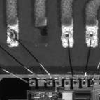
1.2.4 Classifi cation

Another important task is the classifi cation of objects observed in im- ages. The classical example of classifi cation is the recognition of char- acters (optical character recognition or short OCR). Figure 1.10a shows a typical industrial OCR application, the recognition of a label on an in- tegrated circuit. Object classifi cation includes also the recognition of diff erent possible positioning of objects for correct handling by a robot. In Fig. 1.10b, connectors are placed in random orientation on a conveyor belt. For proper pick up and handling, whether the front or rear side of the connector is seen must also be detected.

The classifi cation of defects is another important application. Fig- ure 1.11 shows a number of typical errors in the inspection of integrated circuits: an incorrectly centered surface mounted resistor (Fig. 1.11a), and broken or missing bond connections (Fig. 1.11b–f).

The application of classifi cation is not restricted to industrial tasks. Figure 1.12 shows some of the most distant galaxies ever imaged by the Hubble telescope. The galaxies have to be separated into diff erent classes due to their shape and color and have to be distinguished from other objects, e. g., stars.

1.2 Examples of Applications                                                         13

 

A                                          b                                          c

D                                          e                                          f

Figure 1.11: Errors in soldering and bonding of integrated circuits. Courtesy of Florian Raisch, Robert Bosch GmbH).

 

 

Figure 1.12: Hubble deep space image: classifi cation of distant galaxies (http: //hubblesite.org/).

14                                                                                      1 Applications and Tools

 

 

Figure 1.13: A hierarchy of digital image processing tasks from image formation to image comprehension. The numbers by the boxes indicate the corresponding chapters of this book.

1.3 Hierarchy of Image Processing Operations                                 15

 

⇐ Предыдущая12345678910Следующая ⇒

Поделиться: