Spatial Representation of Digital Images

Pixel and Voxel

Images constitute a spatial distribution of the irradiance at a plane. Mathematically speaking, the spatial irradiance distribution can be de- scribed as a continuous function of two spatial variables:

E(x₁, x₂) = E( x ). (2.1)

Computers cannot handle continuous images but only arrays of digi- tal numbers. Thus it is required to represent images as two-dimensional arrays of points. A point on the 2-D grid is called a pixel or pel. Both words are abbreviations of the word picture element. A pixel represents the irradiance at the corresponding grid position. In the simplest case, the pixels are located on a rectangular grid. The position of the pixel

ISBN 3–540–67754–2 All rights of reproduction in any form reserved.

30 2 Image Representation

Figure 2.1: Representation of digital images by arrays of discrete points on a rectangular grid: a 2-D image, b 3-D image.

−

× −

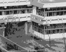
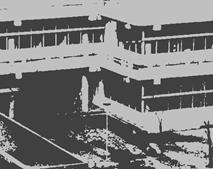
is given in the common notation for matrices. The ﬁ rst index, m, de- notes the position of the row, the second, n, the position of the column (Fig. 2.1a). If the digital image contains M N pixels, i. e., is represented by an M N matrix, the index n runs from 0 to N 1, and the index m from 0 to M 1. M gives the number of rows, N the number of columns. In accordance with the matrix notation, the vertical axis (y axis) runs from top to bottom and not vice versa as it is common in graphs. The horizontal axis (x axis) runs as usual from left to right.

Each pixel represents not just a point in the image but rather a rectan- gular region, the elementary cell of the grid. The value associated with the pixel must represent the average irradiance in the corresponding cell in an appropriate way. Figure 2.2 shows one and the same image repre- sented with a diﬀ erent number of pixels as indicated in the legend. With large pixel sizes (Fig. 2.2a, b), not only is the spatial resolution poor, but the gray value discontinuities at pixel edges appear as disturbing arti- facts distracting us from the content of the image. As the pixels become smaller, the eﬀ ect becomes less pronounced up to the point where we get the impression of a spatially continuous image. This happens when the pixels become smaller than the spatial resolution of our visual sys- tem. You can convince yourself of this relation by observing Fig. 2.2 from diﬀ erent distances.

How many pixels are suﬃ cient? There is no general answer to this question. For visual observation of a digital image, the pixel size should be smaller than the spatial resolution of the visual system from a nomi- nal observer distance. For a given task the pixel size should be smaller than the ﬁ nest scales of the objects that we want to study. We generally ﬁ nd, however, that it is the available sensor technology (see Section 1.7.1)

2.2 Spatial Representation of Digital Images 31

A b

C d

Figure 2.2: Digital images consist of pixels. On a square grid, each pixel rep- resents a square region of the image. The ﬁ gure shows the same image with a

× × × ×

3 4, b 12 16, c 48 64, and d 192 256 pixels. If the image contains suﬃ - cient pixels, it appears to be continuous.

that limits the number of pixels rather than the demands from the appli- cations. Even a high-resolution sensor array with 1000 1000 elements has a relative spatial resolution of only 10− 3. This is a rather poor resolu- tion compared to other measurements such as those of length, electrical voltage or frequency, which can be performed with relative resolutions of far beyond 10− 6. However, these techniques provide only a measure- ment at a single point, while a 1000 1000 image contains one million points. Thus we obtain an insight into the spatial variations of a signal. If we take image sequences, also the temporal changes and, thus, the kinematics and dynamics of the studied object become apparent. In this way, images open up a whole new world of information.

A rectangular grid is only the simplest geometry for a digital image. Other geometrical arrangements of the pixels and geometric forms of the elementary cells are possible. Finding the possible conﬁ gurations is the 2-D analogue of the classiﬁ cation of crystal structure in 3-D space, a subject familiar to solid state physicists, mineralogists, and chemists. Crystals show periodic 3-Dpatterns of the arrangements of their atoms,

32 2 Image Representation

a b c

Figure 2.3: The three possible regular grids in 2-D: a triangular grid, b square grid, c hexagonal grid.

a b c

Figure 2.4: Neighborhoods on a rectangular grid: a 4-neighborhood and b 8- neighborhood. c The black region counts as one object (connected region) in an 8-neighborhood but as two objects in a 4-neighborhood.

ions, or molecules which can be classiﬁ ed by their symmetries and the geometry of the elementary cell. In 2-D, classiﬁ cation of digital grids is much simpler than in 3-D. If we consider only regular polygons, we have only three possibilities: triangles, squares, and hexagons (Fig. 2.3).

The 3-D spaces (and even higher-dimensional spaces) are also of in- terest in image processing. In three-dimensional images a pixel turns into a voxel, an abbreviation of volume element. On a rectangular grid, each voxel represents the mean gray value of a cuboid. The position of a voxel is given by three indices. The ﬁ rst, k, denotes the depth, m the row, and n the column (Fig. 2.1b). A Cartesian grid, i. e., hypercubic pixel, is the most general solution for digital data since it is the only geometry that can easily be extended to arbitrary dimensions.

Neighborhood Relations

An important property of discrete images is their neighborhood relations since they deﬁ ne what we will regard as a connected region and therefore as a digital object. A rectangular grid in two dimensions shows the unfortunate fact, that there are two possible ways to deﬁ ne neighboring pixels (Fig. 2.4a, b). We can regard pixels as neighbors either when they

2.2 Spatial Representation of Digital Images 33

A b c

Figure 2.5: The three types of neighborhoods on a 3-D cubic grid. a 6- neighborhood: voxels with joint faces; b 18-neighborhood: voxels with joint edges; c 26-neighborhood: voxels with joint corners.

have a joint edge or when they have at least one joint corner. Thus a pixel has four or eight neighbors and we speak of a 4-neighborhood or an 8-neighborhood.

Both types of neighborhood are needed for a proper deﬁ nition of objects as connected regions. A region or an object is called connected when we can reach any pixel in the region by walking from one neighbor- ing pixel to the next. The black object shown in Fig. 2.4c is one object in the 8-neighborhood, but constitutes two objects in the 4-neighborhood. The white background, however, shows the same property. Thus we have either two connected regions in the 8-neigborhood crossing each other or two separated regions in the 4-neighborhood. This inconsis- tency can be overcome if we declare the objects as 4-neighboring and the background as 8-neighboring, or vice versa.

These complications occur not only with a rectangular grid. With a triangular grid we can deﬁ ne a 3-neighborhood and a 12-neighborhood where the neighbors have either a common edge or a common corner, respectively (Fig. 2.3a). On a hexagonal grid, however, we can only deﬁ ne a 6-neighborhood because pixels which have a joint corner, but no joint edge, do not exist. Neighboring pixels always have one joint edge and two joint corners. Despite this advantage, hexagonal grids are hardly used in image processing, as the imaging sensors generate pixels on a rectangular grid. The photosensors on the retina in the human eye, however, have a more hexagonal shape [193].

In three dimensions, the neighborhood relations are more complex. Now, there are three ways to deﬁ ne a neighbor: voxels with joint faces, joint edges, and joint corners. These deﬁ nitions result in a 6-neighbor- hood, an 18-neighborhood, and a 26-neighborhood, respectively (Fig. 2.5). Again, we are forced to deﬁ ne two diﬀ erent neighborhoods for objects and the background in order to achieve a consistent deﬁ nition of con- nected regions. The objects and background must be a 6-neighborhood and a 26-neighborhood, respectively, or vice versa.

34 2 Image Representation

Discrete Geometry

The discrete nature of digital images makes it necessary to redeﬁ ne el- ementary geometrical properties such as distance, slope of a line, and coordinate transforms such as translation, rotation, and scaling. These quantities are required for the deﬁ nition and measurement of geometric parameters of object in digital images.

In order to discuss the discrete geometry properly, we introduce the grid vector that represents the position of the pixel. The following dis- cussion is restricted to rectangular grids. The grid vector is deﬁ ned in 2-D, 3-D, and 4-D spatiotemporal images as

Σ n∆ x Σ

 n∆ x 

r m, n =

m∆ y

, r _{l, m, n} =  m∆ y

m∆ y

 , r k, l, m, n = 

 . (2.2)

 l∆ z 

l∆ z





 k∆ t 

To measure distances, it is still possible to transfer the Euclidian dis- tance from continuous space to a discrete grid with the deﬁ nition

1/2

d_e( r, r ') = ⊗ r − r '⊗ = Σ (n − n')2∆ x2 + (m − m')2∆ y2Σ . (2.3)

Equivalent deﬁ nitions can be given for higher dimensions. In digital images two other metrics have often been used. The city block distance

d_b( r, r ') = |n − n'|+ |m − m'| (2.4)

gives the length of a path, if we can only walk in horizontal and verti- cal directions (4-neighborhood). In contrast, the chess board distance is deﬁ ned as the maximum of the horizontal and vertical distance

d_c( r, r ') = max(|n − n'|, |m − m'|). (2.5)

For practical applications, only the Euclidian distance is relevant. It is the only metric on digital images that preserves the isotropy of the con- tinuous space. With the city block distance, for example, distances in the direction of the diagonals are longer than the Euclidean distance. The curve with equal distances to a point is not a circle but a diamond-shape curve, a square tilted by 45°.

Translation on a discrete grid is only deﬁ ned in multiples of the pixel or voxel distances

r 'm, n = r _m,_n + t _m', n', (2.6)

i. e., by addition of a grid vector t _m', n'.

Likewise, scaling is possible only for integer multiples of the scaling factor by taking every qth pixel on every pth line. Since this discrete scaling operation subsamples the grid, it remains to be seen whether the scaled version of the image is still a valid representation.

2.2 Spatial Representation of Digital Images 35

Figure 2.6: A discrete line is only well deﬁ ned in the directions of axes and di- agonals. In all other directions, a line appears as a staircase-like jagged pixel sequence.

Rotation on a discrete grid is not possible except for some trivial angles. The condition is that all points of the rotated grid coincide with the grid points. On a rectangular grid, only rotations by multiples of 180° are possible, on a square grid by multiples of 90°, and on a hexagonal grid by multiples of 60°.

Generally, the correct representation even of simple geometric ob- jects such as lines and circles is not clear. Lines are well-deﬁ ned only for angles with values of multiples of 45°, whereas for all other directions they appear as jagged, staircase-like sequences of pixels (Fig. 2.6).

All these limitations of digital geometry cause errors in the position, size, and orientation of objects. It is necessary to investigate the conse- quences of these errors for subsequent processing carefully.

Quantization

For use with a computer, the measured irradiance at the image plane must be mapped onto a limited number Q of discrete gray values. This process is called quantization. The number of required quantization levels in image processing can be discussed with respect to two criteria. First, we may argue that no gray value steps should be recognized by our visual system, just as we do not see the individual pixels in digital images. Figure 2.7 shows images quantized with 2 to 16 levels of gray values. It can be seen clearly that a low number of gray values leads to false edges and makes it very diﬃ cult to recognize objects that show slow spatial variation in gray values. In printed images, 16 levels of gray values seem to be suﬃ cient, but on a monitor we would still be able to

see the gray value steps.

Generally, image data are quantized into 256 gray values. Then each pixel occupies 8 bits or one byte. This bit size is well adapted to the architecture of standard computers that can address memory bytewise. Furthermore, the resolution is good enough to give us the illusion of a

36 2 Image Representation

A b

C d

Figure 2.7: Illustration of quantization. The same image is shown with diﬀ erent quantization levels: a 16, b 8, c 4, d 2. Too few quantization levels produce false edges and make features with low contrast partly or totally disappear.

continuous change in the gray values, since the relative intensity resolu- tion of our visual system is no better than about 2 %.

The other criterion is related to the imaging task. For a simple ap- plication in machine vision, where homogeneously illuminated objects must be detected and measured, only two quantization levels, i. e., a bi- nary image, may be suﬃ cient. Other applications such as imaging spec- troscopy or medical diagnosis with x-ray images require the resolution of faint changes in intensity. Then the standard 8-bit resolution would be too coarse.

2.2.5 Signed Representation of Images‡

Normally we think of “brightness” (irradiance or radiance) as a positive quantity. Consequently, it appears natural to represent it by unsigned numbers ranging in an 8-bit representation, for example, from 0 to 255. This representation causes problems, however, as soon as we perform arithmetic operations with images. Subtracting two images is a simple example that can produce negative numbers. Since negative gray values cannot be represented, they wrap around

2.2 Spatial Representation of Digital Images 37

Figure 2.8: The context determines how “bright” we perceive an object to be. Both squares have the same brightness, but the square on the dark background appears brighter than the square on the light background. The two squares only appear equally bright if they touch each other.

− =

−

and appear as large positive values. The number 1, for example, results in the positive value 255 given that 1 modulo 256 255. Thus we are confronted with the problem of two diﬀ erent representations of gray values, as unsigned and signed 8-bit numbers. Correspondingly, we must have several versions of each algorithm, one for unsigned gray values, one for signed values, and others for mixed cases.

One solution to this problem is to handle gray values always as signed num- bers. In an 8-bit representation, we can convert unsigned numbers into signed numbers by subtracting 128:

q' = (q − 128) mod 256, 0 ≤ q< 256. (2.7)

Then the mean gray value intensity of 128 becomes the gray value zero and gray values lower than this mean value become negative. Essentially, we regard gray values in this representation as a deviation from a mean value.

This operation converts unsigned gray values to signed gray values which can be stored and processed as such. Only for display must we convert the gray values again to unsigned values by the inverse point operation

q = (q' + 128) mod 256, − 128 ≤ q' < 128, (2.8)

which is the same operation as in Eq. (2.7) since all calculations are performed modulo 256.

⇐ Предыдущая 3 4 5 6 789 10 11 12 Следующая ⇒

Последнее изменение этой страницы: 2019-05-04; Просмотров: 174; Нарушение авторского права страницы