Functions of Multiple Random Variables

In extension to the discussion of functions of a single RV in Section 3.2.3, we can express the mean of a function of multiple random variables g' = p(g₁, g₂,..., g_P ) directly from the joint PDF:

∞

Eg' =

∫ p(g₁, g₂,..., g_P )f (g₁, g₂,..., g_P )dg₁dg₂... dg_P.                                (3.22)

− ∞

From this general relation it follows that the mean of any linear function

 

.

P

g' =   a_pg_p                                               (3.23)

p=1

is given as the linear combination of the means of the RVs g_p:

 P                P            . Σ

p=1

p=1

E  . a_pg_p =. a_pE  g_p.                                  (3.24)

 

Note that this is a very general result. We did not assume that the RVs are independent, and this is not dependent on the type of the PDF. As a special case Eq. (3.24) includes the simple relations

E(g₁ + g₂) = Eg₁ + Eg₂,              E(g₁ + a) = Eg₁ + a.                  (3.25)

×

The variance of functions of multiple RVs cannot be computed that easy even in the linear case. Let g be a vector of P RVs, g ' a vector of Q RVs that is a linear combination of the P RVs g, M a Q P matrix of coeffi cients, and a a column vector with Q coeffi cients. Then

g ' = Mg + a with E( g ') = M E( g ) + a                                (3.26)

=

in extension to Eq. (3.24). If P Q, Eq. (3.26) can be interpreted as a coordinate transformation in a P-dimensional vector space. Therefore it is not surprising that the symmetric covariance matrix transforms as a second-order tensor [134]:

cov( g ') = M   cov( g ) M T .                                       (3.27)

To illustrate the application of Eq. (3.27), we apply it to several exam- ples. First, we discuss the computation of the variance of the mean g of

3.3 Multiple Random Variables                                                        85

P RVs with the same mean and variance σ 2. We assume that the RVs are uncorrelated. Then the matrix M and the covariance matrix cov g are



σ 2  0     ...  0

1                                                                  0   σ 2...  0

M = [1, 1, 1,..., 1]     and cov( g ) = 

 

                                                          



2

 = σ I.

.   .   ....

                          

 0  0  ... σ 2 

Using these expressions in Eq. (3.27) yields

σ 2 = 1 σ 2.                                                  (3.28)

g       N

g

=       =

Thus the variance σ 2 is proportional to N− 1 and the standard deviation σ _g decreases only with N− 1/2. This means that we must take four times as many measurements in order to double the precision of the measure- ment of the mean. This is not the case for correlated RVs. If the RVs are fully correlated (r_pq 1, C_pq  σ 2), according to Eq. (3.27), the variance of the mean is equal to the variance of the individual RVs. In this case it is not possible to reduce the variance by averaging.

p

In a slight variation, we take P uncorrelated RVs with unequal vari- ances σ 2 and compute the variance of the sum of the RVs. From Eq. (3.25), we know already that the mean of the sum is equal to the sum of the means (even for correlated RVs). Similar as for the previous example, it can be shown that for uncorrelated RVs the variance of the sum is also the sum of the individual variances:

P                   P

var. g_p =. var g_p.                                       (3.29)

p=1              p=1

As a third example we take Q RVs g_q'  that are a linear combination

of the P uncorrelated RVs g_p with equal variance σ 2:

q

g_q' = a T  g.                                                    (3.30)

q

×

Then the vectors a T form the rows of the Q               P matrix M in Eq. (3.26) and the covariance matrix of g ' results according to Eq. (3.27) in

1 T

1 T

1 T

 a T a ₁ a T a ₂... a T a _Q 

2         T           2 a 1 a 2 a 2 a 2... a 2 a Q

cov( g ') = σ MM = σ 

 

                  

 .    (3.31)

.         .         ....

                                       

 a T a _Q a T a _Q... a T a _Q 

q

From this equation, we can learn two things. First, the variance of the RV g_q'  is given by a T  a _q, i. e., the sum of the squares of the coeffi cients

q

σ 2(g_q' ) = σ 2 a T  a _q.                                               (3.32)

86                                                                         3 Random Variables and Fields

 

p

Second, although the RVs g_p are uncorrelated, two RVs g_p'  and g_q' are only uncorrelated if the scalar product of the coeffi cient vectors, a T a _q, is zero, i. e., the coeffi cient vectors are orthogonal. Thus, only orthogonal transform matrixes M in Eq. (3.26) leave uncorrelated RVs uncorrelated.

The above analysis of the variance for functions of multiple RVs can be extended to nonlinear functions provided that the function is suffi - ciently linear around the mean value. As in Section 3.2.3, we expand the nonlinear function p_q( g ) into a Taylor series around the mean value:

. p

P  ∂ p_q

gp'

= p_q( g ) ≈ p_q( µ ) +       ∂ g (g_p − µ_p).                       (3.33)

p=1

×

We compare this equation with Eq. (3.26) and fi nd that the Q                     P matrix

M has to be replaced by the matrix J





J = 



∂ p₁

∂ g₁

∂ p₂

∂ g₁

∂ p₁

∂ g₂

∂ p₂

∂ g₂

... ∂ p 1

∂ g_P

... ∂ p 2

∂ g_P

 





 ,                        (3.34)



.       .       .  .

.    .      ..

 

 

                                  

∂ p_Q

∂ g₁

∂ p_Q

∂ g₂

... ∂ p Q

∂ g_P

=

known as the Jacobian matrix of the transform g '                  p ( g ). Thus the covariance of g ' is given by

cov( g ') ≈ J cov( g ) J T .                                         (3.35)

= +

∞

Finally, we discuss the PDFs of function of multiple RVs. We restrict the discussion to two simple cases. First, we consider the addition of two RVs. If two RVs g₁ and g₂ are independent, the resulting probability density function of an additive superposition g g₁ g₂ is given by the convolution integral

p_g(g) =

∫ p_g1 (g')p_g2 (g − g')dg'.                                   (3.36)

− ∞

=            = −

This general property results from the multiplicative nature of the su- perposition of probabilities. The probability p_g(g) to measure the value g is the product of the probabilities to measure g₁ g' and g₂ g g'. The integral in Eq. (3.36) itself is required because we have to consider all combinations of values that lead to a sum g.

=    +

Second, the same procedure can be applied to the multiplication of two RVs if the multiplication of two variables is transformed into an addition by applying the logarithm: ln g ln g₁ ln g₂. The PDFs of the logarithm of an RV can be computed using Eq. (3.9).

3.4 Probability Density Functions                                                    87

 

A                                                                   b

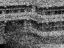
C                                                                   d

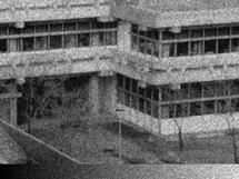
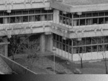
Figure 3.2: Simulation of low-light images with Poisson noise that have collected maximal a 3, b 10, c 100, and d 1000 electrons. Note the linear intensity wedge at the bottom of images c and d .

 

⇐ Предыдущая13141516171819202122Следующая ⇒

Поделиться: