
|
Архитектура Аудит Военная наука Иностранные языки Медицина Металлургия Метрология Образование Политология Производство Психология Стандартизация Технологии |
|
|
Архитектура Аудит Военная наука Иностранные языки Медицина Металлургия Метрология Образование Политология Производство Психология Стандартизация Технологии |
Interactive Gray Value Evaluation
Homogeneous point operators implemented via look-up tables are a very useful tool for inspecting images. As the look-up table operations work in real-time, images can be manipulated interactively. If only the output look-up table is changed, the original image content remains unchanged. Here, we demonstrate typical tasks.
Evaluating and Optimizing Illumination. With the naked eye, we can hardly estimate the homogeneity of an illuminated area as demonstrated 250 10 Pixel Processing
q
Figure 10.3: Illustration of a nonlinear look-up table with mapping of multiple values onto one and missing output value leading to uneven steps.
in Fig. 10.4a, b. A histogram reveals the gray scale distribution but not its spatial variation (Fig. 10.4c, d). Therefore, a histogram is not of much help for optimizing the illumination interactively. We need to mark gray scales such that absolute gray levels become perceivable for the human eye. If the radiance distribution is continuous, it is suffi cient to use equidensities. This technique uses a staircase type of homogeneous point operation by mapping a certain range of gray scales onto one. This point operation is achieved by zeroing the p least signifi cant bits with a logical and operation:
q' = P (q) = q ∧ (2p − 1), (10.9)
Another way to mark absolute gray values is the so-called pseudo- color image that has already been discussed in Section 10.2.2. With this technique, a gray level q is mapped onto an RGB triple for display. As color is much better recognized by the eye, it helps reveal absolute gray levels.
Detection of Underfl ow and Overfl ow. Under- and overfl ows of the gray values of a digitized image often go unnoticed and cause a serious bias in further processing, for instance for mean gray values of objects or the center of gravity of an object. In most cases, such areas cannot 10.2 Homogeneous Point Operations 251
b
1500
1000
500
0 160 170 180 190 200 210 220
C d
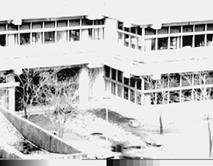
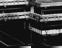
Figure 10.4: a The irradiance is gradually decreasing from the top to the bot- tom, which is almost not recognized by the eye. The gray scale of this fl oating- point image computed by averaging over 100 images ranges from 160 to 200. b Histogram of a; c and d (contrast enhanced, gray scale 184–200): Edges ar- tifi cially produced by a staircase LUT with a step height of 1.0 and 2.0 make contours of constant irradiance easily visible.
be detected directly. They may only become apparent in textured ar- eas when the texture is bleached out. Over and underfl ow are detected easily in histograms by strong peaks at the minimum and/or maximum gray values (Fig. 10.5). With pseudocolor mapping, the few lowest and highest gray values could be displayed, for example, in blue and red, re- spectively. Then, gray values dangerously close to the limits immediately pop out of the image and can be avoided by correcting the illumination lens aperture or gain of the video input circuit of the frame grabber.
Contrast enhancement. Because of poor illumination conditions, it of- ten happens that images are underexposed. Then, the image is too dark and of low contrast (Fig. 10.6a). The histogram (Fig. 10.6b) shows that the image contains only a small range of gray values at low gray values. The appearance of the image improves considerably if we apply a point operation which maps a small grayscale range to the full contrast range 252 10 Pixel Processing
a
1500
1000
500
c
5000 4000 3000 2000 1000 0
Figure 10.5: Detection of underfl ow and overfl ow in digitized images by his- tograms; a image with underfl ow and b its histogram; c image with overfl ow and d its histogram.
The image quality can be improved. The best way is to increase the object irradiance by using a more powerful light source or a better design of the illumination setup. If this is not possible, we can still increase the gain of the analog video amplifi er. All modern image processing boards include an amplifi er whose gain and off set can be set by software (see Figs. 10.1 and 10.2). By increasing the gain, the brightness and resolution of the image improve, but at the expense of an increased noise level.
Contrast Stretching. It is often of interest to analyze faint irradiance diff erences which are beyond the resolution of the human visual system or the display equipment used. This is especially the case if images are printed. In order to observe faint diff erences, we stretch a small gray scale range of interest to the full range available. All gray values outside this range are set to the minimum or maximum value. This operation 10.2 Homogeneous Point Operations 253
b
25000 20000 15000 10000 5000
d
25000 20000 15000 10000 5000 0
Figure 10.6: Contrast enhancement; a underexposed image and b its histogram; c interactively contrast enhanced image and d its histogram.
requires that the gray values of the object of interest fall into the range selected for contrast stretching. An example of contrast stretching is shown in Fig. 10.7a, b. The wedge at the bottom of the images, rang- ing from 0 to 255, directly shows which part of the gray scale range is contrast enhanced.
Range Compression. In comparison to the human visual system, a digital image has a considerably smaller dynamical range. If a minimum resolution of 10 % is demanded, the gray values must not be lower than
255γ 254 10 Pixel Processing
A b
C d
Figure 10.7: b – d Contrast stretching of the image shown in a. The stretched range can be read from the transformation of the gray scale wedge at the bottom of the image.
The factors in Eq. (10.10) are chosen such that a range of [0, 255] is mapped onto itself. This transformation allows a larger dynamic range to be recognized at the cost of resolution in the bright parts of the image. The dark parts become brighter and show more details. This contrast transformation is better adapted to the logarithmic characteristics of the human visual system. An image presented with diff erent gamma factors is shown in Fig. 10.8.
Noise Variance Equalization. From Section 3.4.5, we know that the variance of the noise generally depends on the image intensity according to
A statistical analysis of images and image operations is, however, much easier if the noise is independent of the gray value. Only then all the error propagation techniques discussed in Section 3.3.3 are valid. Thus we need to apply a nonlinear gray value transform h(g) in such a way that the noise variance becomes constant. In fi rst order, the vari- 10.2 Homogeneous Point Operations 255
A b
C d
Figure 10.8: Presentation of an image with diff erent gamma values: a 0.5, b 0.7, c 1.0, and d 2.0.
σ 2(g) Integration yields
g h(g) = σ h∫
dg'
0 σ 2(g') The two free parameters σ h and C can, for instance, be used to fi t the values of h into a suitable interval. With the linear variance function Eq. (10.11), the integral in Eq. (10.13) yields
256 10 Pixel Processing
A b
Figure 10.9: Noise reduction by image averaging: a single thermal image of small temperature fl uctuations on the water surface cooled by evaporation; b same, averaged over 16 images; the full gray value range corresponds to a tem- perature range of 1.1 K.
 2σ h 2σ h
h(g) = √ α , g. (10.15) 10.3 Inhomogeneous Point Operations† Homogeneous point operations are only a subclass of point operators. In general, a point operation depends also on the position of the pixel in the image. Such an operation is called an inhomogeneous point opera- tion. Inhomogeneous point operations are mostly related to calibration procedures. Generally, the computation of an inhomogeneous point op- eration is much more time consuming than the computation of a homo- geneous point operation. We cannot use look-up tables since the point operation depends on the pixel position and we are forced to calculate the function for each pixel. The subtraction of a background image without objects or illumina- tion is a simple example of an inhomogeneous point operation which is written as: Gm' n = Pmn(Gmn) = Gmn − Bmn, (10.16) where Bmn is the background image.
Image Averaging One of the simplest inhomogeneous point operations is image averag- ing. There are a number of imaging sensors available which show a 10.3 Inhomogeneous Point Operations† 257
considerable noise level. Prominent examples include thermal imaging (Section 6.4.1) and all sensor types such as slow-scan CCD imagers or image amplifi ers where only a limited number of photons are collected. Figure 10.9a shows the temperature diff erences at the water surface of a wind-wave facility cooled at 1.8 m/s wind speed by evaporation. Be- cause of a substantial noise level, the small temperature fl uctuations can hardly be detected. Taking the mean over several images signifi cantly reduces the noise level (Fig. 10.9b). The error of the mean (Section 3.3.3) taken from N samples is given
σ 2 1
N
= √ If we take the average of N images, the noise level is reduced by 1/ N compared to a single image. Taking the mean over 16 images thus re- duces the noise level by a factor of four. Equation (10.17) is only valid, however, if the standard deviation σ g is signifi cantly larger than the standard deviation related to the quantization (Section 9.4).
|
Последнее изменение этой страницы: 2019-05-04; Просмотров: 216; Нарушение авторского права страницы
 P(q)
P(q)
 a
a  2000
2000

 b
b  d
d  6000
6000 a
a  30000
30000 c
c  30000
30000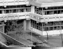


 + C. (10.13)


