Two-Point Radiometric Calibration

The simple ratio imaging described above is not applicable if also a non- zero inhomogeneous background has to be corrected for, as caused, for instance, by the fi xed pattern noise of a CCD sensor. In this case, two reference images are required. This technique is also applied for a sim- ple two-point radiometric calibration of an imaging sensor with a linear response. Some image measuring tasks require an absolute or relative radiometric calibration. Once such a calibration is obtained, we can infer the radiance of the objects from the measured gray values.

First, we take a dark image B without any illumination. Second, we take a reference image R with an object of constant radiance, e. g., by looking into an integrating sphere. Then, a normalized image corrected for both the fi xed pattern noise and inhomogeneous sensitivity is given by

=

G ' c G − B  .                                              (10.19)

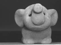
R − B

Fig. 10.11 shows a contrast-enhanced dark image and reference image of a CCD camera with analog output. Typical signal distortions can be observed. The signal oscillation at the left edge of the dark image results from an electronic interference, while the dark blobs in the reference image are caused by dust on the glass window in front of the sensor. The improvement due to the radiometric calibration can clearly be seen in Fig. 10.12.

260                                                                                               10 Pixel Processing

 

A                                                                   b

Figure 10.12: Two-point radiometric calibration with the dark and reference image from Fig. 10.11: a original image and b calibrated image; in the calibrated image the dark spots caused by dust are no longer visible.

 

 

10.3.4 Nonlinear Radiometric Calibration‡

Sometimes, the quantity to be measured by an imaging sensor is related in a nonlinear way to the measured gray value. An obvious example is thermog- raphy. In such cases a nonlinear radiometric calibration is required. Here, the temperature of the emitted object is determined from its radiance using Planck’s equations (Section 6.4.1).

We will give a practical calibration procedure for ambient temperatures. Be- cause of the nonlinear relation between radiance and temperature, a simple two-point calibration with linear interpolation is not suffi cient. Hauß ecker [63] showed that a quadratic relation is accurate enough for a small temperature range, say from 0 to 40° centigrade. Therefore, three calibration temperatures are required, which are provided by a temperature-regulated blackbody calibra- tion unit.

The calibration delivers three calibration images G ₁, G ₂, and G ₃ with known temperatures T₁, T₂, and T₃. The temperature image T of an arbitrary image G can be computed by quadratic interpolation as

 

with

T   ∆ G ₂ · ∆ G ₃

=

∆ G ₂₁ · ∆ G ₃₁

T  ∆ G ₁ · ∆ G ₃

− 1

∆ G ₂₁ · ∆ G ₃₂

T  ∆ G ₁ · ∆ G ₂

+2

∆ G ₃₁ · ∆ G ₃₂

 

T₃,            (10.20)

∆ G _k = G − G _k        and    ∆ G _kl = G _k − G _l.                       (10.21)

·

The symbol indicates pointwise multiplication of the images in order to dis- tinguish it from matrix multiplication. Figure 10.13a, b, and c shows three cali- bration images. The infrared camera looks at the calibration target via a mirror which limits the fi eld of view at the edges of the images. This is the reason for the sharp temperature changes seen at the image borders in Fig. 10.13a, c. The calibration procedure removes the residual inhomogeneities (Fig. 10.13d, f) that show up in the original images.

10.3 Inhomogeneous Point Operations†                                                         261

 

A                                           b                                           c

D                                           e                                           f

Figure 10.13: Three-point calibration of infrared temperature images: a – c show images of calibration targets made out of aluminum blocks at temperatures of 13.06, 17.62, and 22.28° centigrade. The images are stretched in contrast to a narrow range of the 12-bit digital output range of the infrared camera: a: 1715– 1740, b: 1925–1950, c: 2200–2230, and show some residual inhomogeneities, especially vertical stripes. d Calibrated image using the three images a – c with quadratic interpolation. e Original and f calibrated image of the temperature microscale fl uctuations at the ocean surface (area about 0.8 × 1.0 m2).

 

Windowing

±

Another important application of inhomogeneous point operations is an operation known as windowing. Before we can calculate the DFT of an image, the image must be multiplied with a window function. If we omit this step, the spectrum will be distorted by the convolution of the image spectrum with the Fourier transform of the box function, the sinc function (see Section 2.3, R5), which causes spectral peaks to become star-like patterns along the coordinate axes in Fourier space (Fig. 10.14b). We can also explain these distortions with the periodic repetition of fi nite-area images, an eff ect that is discussed in conjunc-

262                                                                                               10 Pixel Processing

 

A                                                                    b

C                                                                    d

Figure 10.14: Eff ect of windowing on the discrete Fourier transform: a original image; b DFT of a without using a window function; c image multiplied with a cosine window; d DFT of c using a cosine window.

 

tion with the sampling theorem in Section 9.2.3. The periodic repetition leads to discontinuities at the horizontal and vertical edges of the image which cause correspondingly high spectral densities along the x and y axes in the Fourier domain.

In order to avoid these distortions, we must multiply the image with a window function that gradually approaches zero towards the edges of the image. An optimum window function should preserve a high spectral resolution and show minimum distortions in the spectrum, that is, its DFT should fall off as fast as possible. These are contradictory require- ments. A good spectral resolution requires a broad window function. Such a window, however, falls off steeply at the edges, causing a slow fall-off of the sidelobes of its spectrum.

A carefully chosen window is crucial for a spectral analysis of time series [119, 133]. However, in digital image processing it is less critical because of the much lower dynamic range of the gray values. A simple

10.4 Multichannel Point Operations‡                                                                263

cosine window

M

N

W_mn = sin. π m Σ sin. π nΣ  ,  0 ≤ m< M, 0 ≤ n< N              (10.22)

 

performs this task well (Fig. 10.14c, d).

=    ·

A direct implementation of the windowing operation is very time con- suming because we would have to calculate the cosine function 2MN times. It is much more effi cient to perform the calculation of the win- dow function once, to store the window image, and to use it then for the calculation of many DFTs. The storage requirements can be reduced by recognizing that the window function Eq. (10.22) is separable, i. e., a product of two functions W_{m, n} cw_m r w_n. Then, we need to calculate only the M plus N values for the column and row functions cw_m and r w_n, respectively. As a result, it is suffi cient to store only the row and column functions. The reduced storage space comes at the expense of an additional multiplication per pixel for the window operation.

 

10.4 Multichannel Point Operations‡

10.4.1 Defi nitions‡

Point operations can be generalized to multichannel point operations in a straight- forward way. The operation still depends only on the values of a single pixel. The only diff erence is that it depends on a vectorial input instead of a scalar input. Likewise, the output image can be a multichannel image. For homoge- neous point operations that do not depend on the position of the pixel in the image, we can write

 

Σ                                     Σ

with

G ' = P ( G )                                                  (10.23)

G '  =     G '0  G '1  ... G 'l  ... G 'L− 1

G = [ G ₀ G ₁... G _k... G _{K− 1}],

 

(10.24)

where G 'l and G _k are the components l and k of the multichannel images G ' and

G with L and K channels, respectively.

An important subclass of multicomponent point operators are linear opera- tions. This means that each component of the multichannel image G ' is a linear combination of the components of the multichannel image G:

.

K− 1

G 'l =     P_lk G _k                                             (10.25)

k=0

where P_lk are constant coeffi cients. Therefore, a general linear multicomponent point operation is given by a matrix (or tensor) of coeffi cients P_lk. Then, we can write Eq. (10.25) in matrix notation as

G ' = PG                                                   (10.26)

where P is the matrix of coeffi cients.

264                                                                                               10 Pixel Processing

 

If the components of the multichannel images in a point operation are not inter- related to each other, all coeffi cients in P except those on the diagonal become zero. For K-channel input and output images, just K diff erent point operations remain, one for each channel. The matrix of point operations fi nally reduces to a standard scalar point operation when the same point operation is applied to each channel of a multi-component image.

For an equal number of output and input images, linear point operations can be interpreted as coordinate transformation. If the matrix of the coeffi cients in Eq. (10.26) has a rank R < K, the multichannel point operation projects the K-dimensional space to an R-dimensional subspace.

Generally, linear multichannel point operations are quite easy to handle as they can be described in a straightforward way with the concepts of linear algebra. For square matrices, for instance, we can easily give the condition when an inverse operation to a multichannel operation exists and compute it. For non- linear multicomponent point operations, the linear coeffi cients in Eqs. (10.25) and (10.26) have to be replaced by nonlinear functions:

G ^'_l = P_l( G ₀, G ₁,..., G _{K− 1})                                           (10.27)

Nonlinear multicomponent point operations cannot be handled in a general way, unlike linear operations. Thus, they must be considered individually. The complexity can be reduced signifi cantly if it is possible to separate a given mul- tichannel point operation into its linear and nonlinear parts.

 

10.4.2 Dyadic Point Operations‡

Operations in which only two images are involved are termed dyadic point op- erations. Dyadic homogeneous point operations can be implemented as LUT operations. Generally, any dyadic image operation can be expressed as

G_m'  n = P(G_mn, H_mn).                                               (10.28)

=

×

If the gray values of the two input images take Q diff erent values, there are Q2 combinations of input parameters and, thus, diff erent output values. Thus, for 8-bit images, 64K values need to be calculated. This is still a quarter less then with a direct computation for each pixel in a 512 512 image. All possible results of the dyadic operation can be stored in a large LUT L with Q2 64K entries in the following manner:

L(2⁸ p + q) = P(p, q), 0 ≤ p, q < Q.                                   (10.29)

The high and low bytes of the LUT address are given by the gray values in the images G and H, respectively.

Some image processing systems contain a 16-bit LUT as a modular processing element. Computation of a dyadic point operation either with a hardware or software LUT is often signifi cantly faster than a direct implementation, espe- cially if the operation is complex. In addition, it is easier to control exceptions such as division by zero or underfl ow and overfl ow.

A dyadic point operation can be used to perform two point operations simul- taneously. The phase and magnitude (r, i) of a complex-valued image, for ex- ample, can be computed simultaneously with one dyadic LUT operation if we

10.5 Geometric Transformations                                                    265

restrict the output to 8 bits as well:

π

r

L(2⁸ r + i) = 2⁸, r 2 + i2 + 128 arctan. i Σ  ,  0 ≤ r, i< Q.                                    (10.30)

 

The magnitude is returned in the high byte and the phase, scaled to the interval

[− 128, 127], in the low byte.

 

⇐ Предыдущая45464748495051525354Следующая ⇒

Поделиться: