Global Smoothness Constraints

⇐ ПредыдущаяСтр 72 из 85Следующая ⇒

One of the most elementary global regularizers is smoothness. For many problems in image processing it makes sense to demand that a quantity to be modeled changes only slowly in space and time. For a segmentation problem this demand means that an object is deﬁ ned just by the fact that it is a connected region with constant or only slowly changing features. Likewise, the depth of a surface and the velocity ﬁ eld of a moving object are continuous at least at most points.

Therefore, we now seek a suitable regularizer R to add to the Lagrange function to force spatially smooth solutions. Such a term requires spatial partial derivatives of the modeled feature. The simplest term, containing only ﬁ rst-order derivatives, for a scalar feature f in a 2-Dimage is

R.f_x, f_yΣ = α 2 .f 2 + f 2Σ = α 2|∇ f |2. (17.18)

x y

For a vector feature f = [f₁, f₂]T

R. f _x, f _yΣ = α 2 .| ∇ f₁|2 + | ∇ f₂|2Σ . (17.19)

In this additional term the partial derivatives emerge as a sum of squares. This means that we evaluate the smoothness term with the same

17.3 Variational Image Modeling† 449

norm (L₂-norm, sum of least squares) as the similarity term. Moreover, in this formulation all partial derivatives are weighted equally. The factor α 2 indicates the relative weight of the smoothness term compared to the similarity term.

The complete least-squares error functional for motion determina- tion including the similarity and smoothing terms is then given by

L. f , f _x, f _yΣ =. f ∇ g + g_tΣ 2 + α 2 .| ∇ f₁|2 + | ∇ f₂|2Σ . (17.20)

Inserting this Lagrange function into the Euler-Lagrange equation (17.9) yields the following diﬀ erential equation:

. ∇ g f + g_tΣ g_x − α 2 .(f₁)_xx + (f₁)_yy Σ = 0

. ∇ g f + g_tΣ g_y − α 2 .(f₂)_xx + (f₂)_yy Σ = 0, or summarized in a vector equation:

(17.21)

∂ t

. ∇ g f + ∂ g Σ ∇ g − α 2∆ f

= 0. (17.22)

similar˛ i¸ ty term r

smoothn˛ ¸ essrterm

It is easy to grasp how the optical ﬂ ow results from this formula. First, imagine that the intensity is changing strongly in a certain direction. The similarity term then becomes dominant over the smoothness term and the velocity will be calculated according to the local optical ﬂ ow. In contrast, if the intensity change is small, the smoothness term becomes dominant. The local velocity will be calculated in such a manner that it is as close as possible to the velocity in the neighborhood. In other words, the ﬂ ow vectors are interpolated from surrounding ﬂ ow vectors.

This process may be illustrated further by an extreme example. Let us consider an object with a constant intensity moving against a black background. Then the similarity term vanishes completely inside the object, while at the border the velocity perpendicular to the border can be calculated just from this term.

This is an old and well-known problem in physics: the problem of how to calculate the potential function (without sinks and sources, ∆ f 0 ) with given boundary conditions at the edge of the object. This equation is known as the Laplacian equation. We can immediately conclude the

form of the solution in areas where the similarity term is zero. As the second-order derivatives are zero, the ﬁ rst-order spatial derivatives are constant. This leads to a modeled feature f that changes linearly in space.

450 17 Regularization and Modeling

17.3.5 Elasticity Models‡

At this point of our discussion, it is useful to discuss an analogous physical problem that gives further insight how similarity and smoothing constraints balance each other. With a physical model these two terms correspond to two types of forces.

Again, we will use the example of optical ﬂ ow determination. We regard the image as painted onto an elastic membrane. Motion will shift the membrane from image to image. Especially nonuniform motion causes a slight expansion or contraction of the membrane. The similarity term acts as an external force that tries to pull the membrane towards the corresponding displacement vector (DV). The inner elastic forces distribute these deformations continuously over the whole membrane, producing a smooth displacement vector ﬁ eld (DVF).

Let us ﬁ rst consider the external forces in more detail. It does not make much sense to set the deformations at those points where we can determine the DV to the estimated displacement without any ﬂ exibility. Instead we allow deviations from the expected displacements which may be larger, the more uncertain the determination of the DV is. Physically, this is similar to a pair of springs whose spring constant is proportional to the certainty with which the displacement can be calculated. The zero point of the spring system is set to the computed displacement vector. As the membrane is two-dimensional, two pairs of springs are required. The direction of the spring system is aligned according to the local orientation (Section 13.3). At an edge, only the displacement normal to the edge can be computed (aperture problem, Section 14.2.2). In this case, only one spring pair is required; a displacement parallel to the edge does not result in a restoring force.

The external spring forces are balanced by the inner elastic forces trying to even out the diﬀ erent deformations. Let us look again at the Euler-Lagrange equation of the optical ﬂ ow (Eq. (17.22)) from this point of view. We can now understand this equation in the following way:

. ∇ g f + g_tΣ ∇ g − α 2∆ f

= 0, (17.23)

extern˛ a¸ l force r intern˛ a¸ l forrce

where α 2 is an elasticity constant. In the expression for the internal forces only second derivatives appear, because a constant gradient of the optical ﬂ ow does not result in net inner forces.

The elasticity features of the membrane are expressed in a single constant. Fur- ther insight into the inner structure of the membrane is given by the Lagrange function (Eq. (17.18)):

L. f , f _x, x Σ = α 2.| ∇ f ₁|2 + | ∇ f |2Σ +. ∇ g f + g_tΣ . (17.24)

T, deforma˛ t¸ ion energy r

–V, po˛ ¸ tential r

The Lagrange function is composed of the potential of the external force as it results from the continuity of the optical ﬂ ow and an energy term related to the inner forces. This term is thus called deformation energy. This energy appears in place of the kinetic energy in the classical example of the Lagrange function for a mass point, as the minimum is not sought in time but in space.

17.4 Controlling Smoothness 451

The deformation energy may be split up into several terms which are closely related to the diﬀ erent modes of deformation:

T. f

Σ = 1 .(f )

+ (f ) Σ +

2  

1 x 2 y

dila˛ t¸ ion r

2 2

(17.25)



.(f₁)_x − (f₂)_yΣ +.(f₁)_y + (f₂)_xΣ +.(f₁)_y − (f₂)_xΣ   .

sh˛ e¸ ar r rota˛ ¸ tion r

Clearly, the elasticity features of the membrane match the kinematics of motion

optimally. Each possible deformation that may occur because of the diﬀ erent modes of 2-Dmotion on the image plane is equally weighted.

Physically, such a membrane makes no sense. The diﬀ erential equation for a real physical membrane is diﬀ erent [39]:

f − (λ + µ) ∇ ( ∇ u ) − µ∆ u = 0. (17.26) The elasticity of a physical membrane is described by the two constants λ and

= − ∇ ∇

µ. λ µ is not possible; as a result, the additional term ( u ) (in compar- ison to the model membrane for the DVF) never vanishes. If there is no cross contraction, λ can only be zero.

With the membrane model, only the elongation is continuous, but not the ﬁ rst- order derivative. Discontinuities occur exactly at the points where external forces are applied to the membrane. This results directly from Eq. (17.22). A locally applied external force corresponds to a δ distribution in the similarity term. Integrating Eq. (17.22), we obtain a discontinuity in the ﬁ rst-order deriv- atives.

These considerations call into question the smoothness constraints considered so far. We know that the motion of planar surface elements does not result in such discontinuities. Smoothness of the ﬁ rst-order derivatives can be forced if we include second-order derivatives in the smoothness term (Eq. (17.22)) or the deformation energy (Eq. (17.24)). Physically, such a model is similar to a thin elastic plate that cannot be folded like a membrane.

Controlling Smoothness

Having discussed the basic properties of smoothness constraints we now turn to the question of how we can adequately treat spatial and tempo- ral discontinuities with this approach. In a segmentation problem, the modeled feature will be discontinuous at the edge of the object. The same is true for the optical ﬂ ow. The smoothness constraint as we have formulated it so far does not allow for discontinuities. We applied a global smoothness constraint and thus obtained a globally smooth ﬁ eld. Thus we need to develop methods that allow us to detect and to model discontinuities adequately.

452 17 Regularization and Modeling

We will ﬁ rst discuss the principal possibilities for varying the minimal problem within the chosen frame. To do so, we rewrite the integral equation for the minimal problem (Eq. (17.6)) using the knowledge about the meaning of the Lagrange function obtained in the last section:

∫ .S( f ) + R( f _xp)Σ

d^W x → Minimum. (17.27)

Ω similar˛ i¸ ty trerm smoothn˛ ¸ ess terrm

In order to incorporate discontinuities, two approaches are possible:

1. Limitation of integration area. The integration area is one of the ways that the problem of discontinuities in the feature f may be solved. If the integration area includes discontinuities, incorrect values are obtained. Thus algorithms must be found that look for edges in f and, as a consequence, restrict the integration area to the segmented areas. Obviously, this is a diﬃ cult iterative procedure. First, the edges in the image itself do not necessarily coincide with the edges in the feature f . Second, before calculating the feature ﬁ eld f only sparse information is available so that a partition is not possible.

2. Modiﬁ cation of smoothness term. Modiﬁ cation of the smoothness term is another way to solve the discontinuity problem. At points where a discontinuity is suspected, the smoothness constraint may be weakened or may even vanish. This allows discontinuities. Again this is an iterative algorithm. The smoothness term must include a control function that switches oﬀ the smoothness constraint in ap- propriate circumstances. This property is called controlled smooth- ness [181].

In the following, we discuss two approaches that modify the integra- tion area for motion determination. The modiﬁ cation of the smoothing term is discussed in detail in Section 17.5.

Integration along Closed Zero-Crossing Curves. Hildreth [68] used the Laplace ﬁ ltered image, and limited any further computations to zero crossings. This approach is motivated by the fact that zero crossings mark the gray value edges (Section 12.2), i. e., the features at which we can compute the velocity component normal to the edge. The big ad- vantage of the approach is that the preselection of promising features considerably decreases any computation required.

By selecting the zero crossings, the smoothness constraint is lim- ited to a certain contour line. This seems useful, as a zero crossing most likely belongs to an object but does not cross object boundaries. However, this is not necessarily the case. If a zero crossing is contained within an object, the velocity along the contour should show no disconti- nuities. Selecting a line instead of an area for the smoothness constraint

17.4 Controlling Smoothness 453

A b

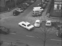
Figure 17.3: Two images of a Hamburg taxi. The video images are from the Computer Science Department at Hamburg University and since then have been used as a test sequence for image sequence processing.

changes the integration region from an area to the line integral along the contour s:

  ( n ¯ f − f_⊥)² + α 2 Σ ((f₁)_s)² + ((f₂)_s)²Σ Σ d s → minimum, (17.28)

where n ¯ is a unit vector normal to the edge and f_⊥ the velocity normal to the edge.

The derivatives of the velocities are computed in the direction of the edge. The component normal to the edge is given directly by the similarity term, while the velocity term parallel to the edge must be inferred from the smoothness constraint all along the edge. Hildreth

[68] computed the solution of the linear equation system resulting from Eq. (17.28) iteratively using the method of conjugate gradients.

Despite its elegance, the edge-oriented method shows signiﬁ cant dis- advantages. It is not certain that a zero crossing is contained within an object. Thus we cannot assume that the optical ﬂ ow ﬁ eld is continuous along the zero crossing. As only edges are used to compute the optical ﬂ ow ﬁ eld, only one component of the displacement vector can be com- puted locally. In this way, all features such as either gray value maxima or gray value corners which allow an unambiguous local determination of a displacement vector are disregarded.

Limitation of Integration to Segmented Regions. A region-oriented approach does not omit such points, but still tries to limit the smooth- ness within objects. Again, zero crossings could be used to separate the image into regions or any other basic segmentation technique (Chap- ter 16). Region-limited smoothness just drops the continuity constraint at the boundaries of the region. The simplest approach to this form of

454 17 Regularization and Modeling

A b

C d

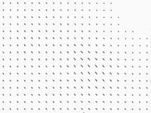
Figure 17.4: Determination of the DVF in the taxi scene (Fig. 17.3) using the method of the dynamic pyramid: a – c three levels of the optical ﬂ ow ﬁ eld using a global smoothness constraint; d ﬁ nal result of the optical ﬂ ow using a region- oriented smoothness constraint; kindly provided by M. Schmidt and J. Dengler, German Cancer Research Center, Heidelberg.

constraint is to limit the integration areas to the diﬀ erent regions and to evaluate them separately.

As expected, a region-limited smoothness constraint results in an op- tical ﬂ ow ﬁ eld with discontinuities at the region’s boundaries (Fig. 17.4d) which is in clear contrast to the globally smooth optical ﬂ ow ﬁ eld in Fig. 17.4c. We immediately recognize the taxi by the boundaries of the optical ﬂ ow.

We also observe, however, that the car is segmented further into re- gions with diﬀ erent optical ﬂ ow ﬁ eld, as shown by the taxi plate on the roof of the car and the back and side windows. The small regions espe- cially show an optical ﬂ ow ﬁ eld signiﬁ cantly diﬀ erent from that in larger regions. Thus a simple region-limited smoothness constraint does not reﬂ ect the fact that there might be separated regions within objects. The optical ﬂ ow ﬁ eld may well be smooth across these boundaries.

17.5 Diﬀ usion Models 455

17.5 Diﬀ usion Models

In this section, we take a new viewpoint of variational image modeling. The least-squares error functional for motion determination (17.20)

∂ t

. ∇ g f + ∂ g Σ ∇ g − α 2∆ f = 0 (17.29)

can be regarded as the stationary solution of a diﬀ usion-reaction sys- tem with homogeneous diﬀ usion if the constant α 2 is identiﬁ ed with a diﬀ usion coeﬃ cient D:

∂ t

f _t = D∆ f − . ∇ g f + ∂ g Σ ∇ g. (17.30)

The standard instationary (partial) diﬀ erential equation for homogeneous diﬀ usion (see Eq. (5.10) in Section 5.2.1) is appended by an additional source term related to the similarity constraint. The source strength is proportional to the deviation from the optical ﬂ ow constraint. Thus this term tends to shift the values for f to meet the optical ﬂ ow constraint.

After this introductionary example, we can formulate the relation between a variational error functional and diﬀ usion-reaction systems in a general way. The Euler-Lagrange equation

∂ _xp L_fxp − L_f = 0 (17.31)

p=1

that minimizes the error functional for the scalar spatiotemporal func- tion f ( x ), x ∈ Ω

Ω

ε (f ) = ∫ L.f, f_xp, x Σ dxW (17.32)

can be regarded as the steady state of the diﬀ usion-reaction system

f_t = ∂ _xp L_fxp − L_f. (17.33)

p=1

In the following we shall discuss an aspect of modeling we have not touched so far — the local modiﬁ cation of the smoothness term. In the language of a diﬀ usion model this means a locally varying diﬀ usion coeﬃ cient in the ﬁ rst-hand term on the right side of Eq. (17.33). From the above discussion we know that to each approach of locally varying diﬀ usion coeﬃ cient, a corresponding variational error functional exists that is minimized by the diﬀ usion-reaction system.

In Section 5.2.1 we discussed a homogeneous diﬀ usion process that generated a multiresolution representation of an image, known as the

456 17 Regularization and Modeling

linear scale space. If the smoothness constraint is made dependent on local properties of the image content such as the gradient, then the in- homogeneous diﬀ usion process leads to the generation of a nonlinear scale space. With respect to modeling, the interesting point here is that a segmentation can be achieved without a similarity term.

17.5.1 Inhomogeneous Diﬀ usion

The simplest approach to a spatially varying smoothing term that takes into account discontinuities is to reduce the diﬀ usion coeﬃ cient at the edges. Thus, the diﬀ usion coeﬃ cient is made dependent on the strength of the edges as given by the magnitude of the gradient

D(f ) = D(| ∇ f |2). (17.34)

With a locally varying diﬀ usion constant the diﬀ usion-reaction system becomes

f_t = ∇. D(| ∇ f |2) ∇ f Σ − L_f. (17.35)

|∇ |

Note that it is incorrect to write D( f 2) ∆ f. This can be seen from the derivation of the instationary diﬀ usion equation in Section 5.2.1.

With Eq. (17.35) the regularization term R in the Lagrange function is

R = R(| ∇ f |2), (17.36)

where the diﬀ usion coeﬃ cient is the derivative of the function R: D R'. This can easily be veriﬁ ed by inserting Eq. (17.36) into Eq. (17.31).

Perona and Malik [136] used the following dependency of the diﬀ u- sion coeﬃ cient on the magnitude of the gradient:

λ 2

D = D₀ |A f |2 + λ 2, (17.37)

|A |,

where λ is an adjustable parameter. For low gradients g λ, D

|A |$

approaches D₀; for high gradients g λ, D tends to zero.

∇

= − .− Σ

As simple and straightforward as this idea appears, it is not without problems. Depending on the functionality of D on g, the diﬀ usion process may become unstable, even resulting in steepening of the edges. A safe way to avoid this problem is to use a regularized gradient obtained from a smoothed version of the image as shown by Weickert [195]. He used

D 1 exp c m . (17.38)

(| ∇ (Br ∗ f )( x )|/λ )m

This equation implies that for small magnitudes of the gradient the dif- fusion coeﬃ cient is constant. At a certain threshold of the magnitude of the gradient, the diﬀ usion coeﬃ cient quickly decreases towards zero.

17.5 Diﬀ usion Models 457

|∇ | = |∇ | =

= =

The higher the exponent m is, the steeper the transition. With the values used by Weickert [195], m 4 and c₄ 3.31488, the diﬀ usion coeﬃ - cient falls from 1 at g /λ 1 to about 0.15 at g /λ 2. Note that a regularized gradient has been chosen in Eq. (17.38), because the gradi- ent is not computed from the image g( x ) directly, but from the image smoothed with a binomial smoothing mask p. A properly chosen reg- ularized gradient stabilizes the inhomogeneous smoothing process and avoids instabilities and steepening of the edges.

A simple explicit discretization of inhomogeneous diﬀ usion uses reg- ularized derivative operators as discussed in Section 12.5. In the ﬁ rst step, a gradient image is computed with the vector operator

D1 . (17.39)

D₂

In the second step, the gradient image is multiplied by the control image R that computes the diﬀ usion coeﬃ cient according to Eq. (17.38) with D₀ = 1:

R· D₁ R· D₂

Σ . (17.40)

The control image is one in constant regions and drops towards small values at the edges. In the third step, the gradient operator is applied a second time

R· D₂

[D₁, D₂] Σ R· D1 Σ = D₁(R· D₁) + D₂(R· D₂). (17.41)

Weickert [195] used a more sophisticated implicit solution scheme. However, the scheme is computationally more expensive and less isotropic than the explicit scheme in Eq. (17.41) if gradient operators are used that are optimized for isotropy as discussed in Section 12.5.5.

An even simpler but only approximate implementation of inhomoge- nous diﬀ usion controls binomial smoothing using the operator

I +R· (B− I). (17.42)

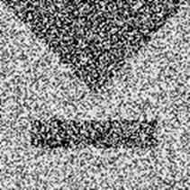
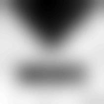
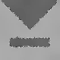
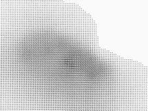
The operator computes the same scalar control image with values between zero and one as in Eq. (17.40).

Figure 17.5 shows the application of inhomogeneous diﬀ usion for segmentation of noisy images. The test image contains a triangle and a rectangle. Standard smoothing signiﬁ cantly suppresses the noise but results in a signiﬁ cant blurring of the edges (Fig. 17.5b). Inhomogenous diﬀ usion does not lead to a blurring of the edges and still results in a perfect segmentation of the square and the triangle (Fig. 17.5c). The only disadvantage is that the edges themselves remain noisy because no smoothing is performed at all there.

458 17 Regularization and Modeling

A b

C d

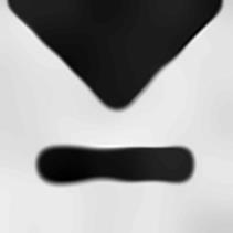
Figure 17.5: a Original, smoothed by b linear diﬀ usion, c inhomogenous but isotropic diﬀ usion, and d anisotropic diﬀ usion. From Weickert [195].

17.5.2 Anisotropic Diﬀ usion

As we have seen in the example discussed at the end of the last section, inhomogeneous diﬀ usion has the signiﬁ cant disadvantage that it stops diﬀ usion completely and in all directions at edges, leaving the edges noisy. However, edges are only blurred by diﬀ usion perpendicular to them; diﬀ usion parallel to them is even advantageous as it stabilizes the edges.

An approach that makes diﬀ usion independent of the direction of edges is known as anisotropic diﬀ usion. With this approach, the ﬂ ux is no longer parallel to the gradient. Therefore, the diﬀ usion can no longer be described by a scalar diﬀ usion coeﬃ cient as in Eq. (5.7). Now,

17.5 Diﬀ usion Models 459

a diﬀ usion tensor is required:

j = − D ∇ f = −  D11 D12

 Σ f1

Σ . (17.43)

 D12 D22  f2

With a diﬀ usion tensor the diﬀ usion-reaction system becomes

f_t = ∇. D ( ∇ f ∇ f T ) ∇ f Σ − L_f (17.44) and the corresponding regularizer is

R = trace R . ∇ f ∇ f T Σ , (17.45)

with D R '. The properties of the diﬀ usion tensor can best be seen if the symmetric tensor is brought into its principal-axis system by a rotation of the coordinate system. Then, Eq. (17.43) reduces to

j ^' = −  D1'

0  Σ f1'

Σ = − Σ D1' f1'

Σ . (17.46)

 0 D2' 

f2'

D2' f2'

The diﬀ usion in the two directions of the axes is now decoupled. The two coeﬃ cients on the diagonal, D₁' and D₂' , are the eigenvalues of the diﬀ usion tensor. By analogy to isotropic diﬀ usion, the general solution for homogeneous anisotropic diﬀ usion can be written as

f (x, t) = 2π σ '(t)σ '(t) exp

− 2σ '(t)

1 .

x'2 Σ

. y'2 Σ

1 2 1

  = =

(17.47)

∗ exp

− 2σ '(t)

∗ f (x, 0)

in the spatial domain with σ ₁'(t) 2D₁' t and σ ₂'(t) 2D₂' t.

This means that anisotropic diﬀ usion is equivalent to cascaded con- volution with two 1-D Gaussian convolution kernels that are steered in the directions of the principal axes of the diﬀ usion tensor. If one of the two eigenvalues of the diﬀ usion tensor is signiﬁ cantly larger than the other, diﬀ usion occurs only in the direction of the corresponding eigen- vector. Thus the gray values are smoothed only in this direction. The spatial widening is — as for any diﬀ usion process — proportional to the square root of the diﬀ usion constant (Eq. (5.15)).

Using this feature of anisotropic diﬀ usion, it is easy to design a dif- fusion process that predominantly smoothes only along edges but not perpendicularly to the edges. The orientation of the edges can be ob- tained, e. g., from the structure tensor (Section 13.3). With the following approach only smoothing across edges is hindered [195]:

D1'

1 exp c m

. Σ = − −

(| ∇ (Br ∗ f )( x )|/λ )m

(17.48)

D2'

= 1.

460 17 Regularization and Modeling

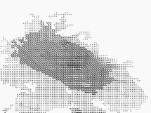
Figure 17.6: Illustration of least-squares linear regression.

As shown by Scharr and Weickert [162], an eﬃ cient and accurate explicit implementation of anisotropic diﬀ usion is again possible with regularized ﬁ rst-order diﬀ erential derivative optimized for minimum anisotropy:

Σ D D1 2

Σ Σ

Σ =

[ , ] R11 R12 D1

R12 R22 D2

(17.49)

with

D₁(R₁₁ · D₁ + R₁₂ · D₂) + D₂(R₁₂ · D₁ + R₂₂ · D₂).

Σ R11 R12

Σ = Σ cos φ sin φ Σ Σ D_x' 0

Σ Σ cos φ − sin φ Σ .

R12 R22

− sin φ cos φ 0 D_y'

sin φ cos φ

The _pq are control images with values between zero and one that steer the diﬀ usion into the direction parallel to edges at each point of the image.

Application of anisotropic diﬀ usion shows that now — in contrast to inhomogeneous diﬀ usion — the edges are also smoothed (Fig. 17.5d). The smoothing along edges has the disadvantage, however, that the cor- ners of the edges are now blurred as with linear diﬀ usion. This did not happen with inhomogeneous diﬀ usion (Fig. 17.5c).

17.6 Discrete Inverse Problems†

In the second part of this chapter, we turn to discrete modeling. Dis- crete modeling can, of course, be derived, by directly discretizing the partial diﬀ erential equations resulting from the variational approach.

17.6 Discrete Inverse Problems† 461

Actually, we have already done this in Section 17.5 by the iterative dis- crete schemes for inhomogeneous and anisotropic diﬀ usion.

However, by developing discrete modeling independently, we gain further insight. Again, we take another point of view of modeling and now regard it as a linear discrete inverse problem. As an introduction, we start with the familiar problem of linear regression and then develop the theory of discrete inverse modeling.

⇐ Предыдущая 67 68 69 70 717273 74 75 76 Следующая ⇒

Последнее изменение этой страницы: 2019-05-04; Просмотров: 177; Нарушение авторского права страницы