Composite Morphological Operators

Opening and Closing

Using the elementary erosion and dilation operations we now develop further useful operations to work on the form of objects. While in the previous section we focused on the general and theoretical aspects of morphological operations, we now concentrate on application.

The erosion operation is useful for removing small objects. However, it has the disadvantage that all the remaining objects shrink in size. We can avoid this eﬀ ect by dilating the image after erosion with the same structure element. This combination of operations is called an opening operation

G ◦ M = ( G ∅ M ) ⊕ M. (18.17)

The opening sieves out all objects which at no point completely con- tain the structure element, but avoids a general shrinking of object size (Fig. 18.2c, d). It is also an ideal operation for removing lines with a thickness smaller than the diameter of the structure element. Note also that the object boundaries become smoother.

In contrast, the dilation operator enlarges objects and closes small holes and cracks. General enlargement of objects by the size of the structure element can be reversed by a following erosion (Fig. 18.3d and e). This combination of operations is called a closing operation

G • M = ( G ⊕ M ) ∅ M. (18.18)

The area change of objects with diﬀ erent operations may be summarized by the following relations:

G ∅ M ⊆ G ◦ M ⊆ G ⊆ G • M ⊆ G ⊕ M. (18.19) Opening and closing are idempotent operations:

G • M = ( G • M ) • M G ◦ M = ( G ◦ M ) ◦ M,

(18.20)

18.4 Composite Morphological Operators 487

A b

C d

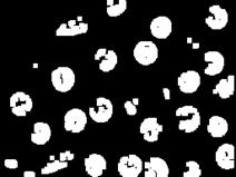
Figure 18.2: Erosion and opening: a original binary image; b erosion with a

3 × 3 mask; c opening with a 3 × 3 mask; d opening with a 5 × 5 mask.

i. e., a second application of a closing and opening with the same struc- ture element does not show any further eﬀ ects.

Hit-Miss Operator

The hit-miss operator originates from the question of whether it is pos- sible to detect objects of a speciﬁ c shape. The erosion operator only removes objects that at no point completely contain the structure ele- ment and thus removes objects of very diﬀ erent shapes. Detection of a speciﬁ c shape requires a combination of two morphological operators. As an example, we discuss the detection of objects containing horizontal rows of three consecutive pixels.

If we erode the image with a 1 3 mask that corresponds to the shape of the object

M ₁ = [11 1], (18.21)

we will remove all objects that are smaller than the target object but retain also all objects that are larger than the mask, i. e., where the shifted mask is a subset of the object G (( M _p ⊆ G ), Fig. 18.4d). Thus, we now

488 18 Morphology

A b

C d

Figure 18.3: Dilation and closing: a original binary image; b dilation with a

3 × 3 mask; c closing with a 3 × 3 mask; d closing with a 5 × 5 mask.

need a second operation to remove all objects larger than the target object.

This can be done by analyzing the background of the original binary image. Thus, we can use as a second step an erosion of the background with a 3 5 mask M ₂ in which all coeﬃ cients are zero except for the pixels in the background, surrounding the object. This is a negative mask for the object:



M ₂ =  

 . (18.22)



1	1	1	1	1
1	0	0	0	1
1	1	1	1	1



⊆

The eroded background then contains all pixels in which the back- ground has the shape of M ₂ or larger ( M ₂ G, Fig. 18.4b). This cor- responds now to objects having the sought shape or a smaller one. As the ﬁ rst erosion obtains all objects equal to or larger than the target, the intersection of the image eroded with M ₁ and the background eroded with M ₂ gives all center pixels of the objects with horizontal rows of three consecutive pixels (Fig. 18.4e). In general, the hit-miss operator is

18.4 Composite Morphological Operators 489

A b c

D e f

× ×

Figure 18.4: Illustration of the hit-miss operator for extracting all objects con- taining horizontal rows of three consecutive pixels: a original image; b back- ground eroded by a 3 5 mask (Eq. (18.22), negative mask of the object); c back- ground eroded by the 3 7 mask (Eq. (18.24)); d object eroded by the 1 3 mask (Eq. (18.21)); e intersection of b and d extracting the objects with horizontal rows of 3 consecutive pixels; f intersection of c and d extracting objects with 3 to 5 horizontal rows of consecutive pixels in a 3 × 7 free background.

deﬁ ned as

G ⊗ ( M ₁, M ₂) = ( G ∅ M ₁) ∩ ( G ∅ M ₂ )

= ( G ∅ M ₁) ∩ ( G ⊕ M ₂)

(18.23)

∩ = ∅

with the condition that M ₁ M ₂ , because otherwise the hit-miss operator would result in the empty set.

With the hit-miss operator, we have a ﬂ exible tool with which we can detect objects of a given speciﬁ c shape. The versatility of the hit-miss operator can easily be demonstrated by using another miss mask



M ₃ =  

 . (18.24)



1	1	1	1	1	1	1
1	0	0	0	0	0	1
1	1	1	1	1	1	1



Erosion of the background with this mask leaves all pixels in the binary image where the union of the mask M ₃ with the object is zero (Fig. 18.4c). This can only be the case for objects with horizontal rows of one to ﬁ ve

490 18 Morphology

consecutive pixels in a 3 7 large background. Thus, the hit-miss oper- ator with M ₁ and M ₃ gives all center pixels of objects with horizontal rows of 3 to 5 consecutive pixels in a 3 7 large background (Fig. 18.4f). As the hit and miss masks of the hit-miss operator are disjunct, they can be combined into one mask using a hit (1), miss (0), and don’t care

(x) notation. The combined mask is marked by 1 where the hit mask is one, by 0 where the miss mask is one, and by x where both masks are zero. Thus, the hit-miss mask for detecting objects with horizontal rows of 3 to 5 consecutive pixels is

M =   0 x 1 1 1 x 0  (18.25)

 0 0 0 0 0 0 0 

0 0 0 0 0 0 0

If a hit-miss mask has no don’t-care pixels, it extracts objects of an exact shape given by the 1-pixels of the mask. If don’t-care pixels are present in the hit-miss mask, the 1-pixels give the minimum and the union of the 1-pixels and don’t-care pixels the maximum of the detected objects.

As another example, the hit-mass mask

 0 0 0 

⊗

M _I =   0 1 0   (18.26)

detects isolated pixels. Thus, the operation G / G M _I removes isolated pixels from a binary image. The / symbol represents the set diﬀ erence operator.

The hit-miss operator detects certain shapes only if the miss mask surrounds the hit mask. If the hit mask touches the edge of the hit-miss mask, only certain shapes at the border of an object are detected. The

hit-miss mask

 x 1 0 

 

M _C =  

1 1 0 , (18.27)

0 0 0

for instance, detects lower right corners of objects.

Thinning

Often it is required to apply an operator that erodes an object but does not break it apart into diﬀ erent pieces. With such an operator, the topol- ogy of the object is preserved and line-like structures can be reduced to a one-pixel thickness. Unfortunately, the erosion operator does not have this feature. It can break an object into pieces.

18.4 Composite Morphological Operators 491

A proper thinning operator, however, must not erode a point under the following conditions: (i) an object must not break into two pieces,

(ii) an end point must not be removed so that the object does not be- come shorter, and (iii) an object must not be deleted. We illustrate this approach with the thinning of an object that has an 8-neighborhood con- nectivity. This corresponds to an erosion by a mask with 4-neighborhood connectivity:

  1 1 1  .

 0 1 0 

0 1 0

The mask contains ﬁ ve nonzero points. Thus there are 25 32 possible binary patterns to which the thinning operator can be applied. Normal erosion would give a nonzero result only when all ﬁ ve points are set. A thinning operator will not erode a point under the following additional conditions:

(i) do not break object into two pieces:

 0 0 0   0 1 0 

  1 1 1  ,  0 1 0   ,

0 0 0   0 1 0

(ii) do not remove end point:

 0 1 0   0 0 0   0 0 0   0 0 0 

0 0 0 

 0 0 0 

 0 1 0 

 0 0 0

  0 1 0  ,  0 1 1  ,  0 1 0  ,  1 1 0   ,

and (iii) do not delete an object:

  0 1 0  .

 0 0 0 

0 0 0

Thus only in 8 out of 16 cases that contain a nonzero central point, it is removed. Because there are only 32 possible patterns, the thinning operator can be implemented in an eﬃ cient way by a 32-entry look-up table with binary output. The addresses for the table are computed in the following way. Each point in the mask corresponds to a bit of the address that is set if the pixel of the binary image on that position is set. The thinning operator is an iterative procedure which can be repeated until no further changes occur. Therefore it makes sense to use a second look-up table that gives a one if the thinning operator results in a change.

In this way, it is easy to count changes and detect when no more changes occur.

492 18 Morphology

A b

C d

Figure 18.5: Boundary extraction with morphological operators: a original bi- nary image; b 8-connected and c 4-connected boundaries extracted with M _b4 and M _b8, respectively, Eq. (18.28); d 8-connected boundary of the background extracted by using Eq. (18.30).

Boundary Extraction

Morphological operators can also be used to extract the boundary of a binary object. This operation is signiﬁ cant as the boundary is a complete yet compact representation of the geometry of an object from which further shape parameters can be extracted, as we discuss later in this chapter.

Boundary points miss at least one of their neighbors. Thus, an ero- sion operator with a mask containing all possible neighbors removes all boundary points. These masks for the 4- and 8-neighborhood are:

 0 1 0   1 1 1 

M _b4 =   1 1 1   and M _b8 =   1 1 1   . (18.28)

18.4 Composite Morphological Operators 493

The boundary is then obtained by the set diﬀ erence (/ operator) between the object and the eroded object:

∂ G = G /( G ∅ M _b )

= G ∩ ( G ∅ M _b)

= G ∩ ( G ¯ ⊕ M _b).

(18.29)

As Eq. (18.29) shows, the boundary is also given as the intersection of the object with the dilated background. Figure 18.5 shows 4- and 8-connected boundaries extracted from binary objects using Eq. (18.28).

The boundary of the background is similarly given by dilating the object and subtracting it:

∂ G _B = ( G ⊕ M _b)/ G. (18.30)

Distance transforms

The boundary consists of all points with a distance zero to the edge of the object. If we apply boundary extraction again to the object eroded with the mask Eq. (18.28), we obtain all points with a distance of one to the boundary of the object. A recursive application of the boundary extraction procedure thus gives the distance of all points of the object to the boundary. Such a transform is called a distance transform and can be written as

b b

D =  Σ (G ∅ Mn− 1)/(G ∅ Mn) · nΣ , (18.31)

n=1

where the operation denotes pointwise multiplication of the binary image of the nth distance contour with the number n.

This straightforward distance transform has two serious ﬂ aws. First, it is a slow iterative procedure. Second, it does not give the preferred Euclidian distance but — depending on the chosen neighborhood con- nectivity — the city block or chess board distance (Section 2.2.3).

Fortunately, fast algorithms are available for computing the Euclidian distance. The Euclidian distance transform is an important transform because it introduces isotropy for morphological operations. All mor- phological operations suﬀ er from the fact that the Euclidian distance is not a natural measure on a rectangular grid. Square-shaped structure elements, for instance, all inherit the chess board distance. Successive dilation with such structure elements makes the objects look more and more like squares, for instance.

The Euclidian distance transform can be used to perform isotropic erosion and dilation operations. For an erosion operation with a radius r, we keep only pixels with a distance greater than r in the object. In

494 18 Morphology

a similar way, an isotropic dilation can be performed by computing a Euclidian distance transform of the background and then an isotropic erosion of the background.

18.5 Further Readings‡

The authoritative source for the theory of morphological image processing is a monograph written by the founders of image morphology, see Serra [168]. The more practical aspects are covered by Jä hne and Hauß ecker [82, Chapter 14] and Soille [175]. Meanwhile morphological image processing is a mature research area with a solid theoretical foundation and a wide range of applications as can be seen from recent conference proceeding, e. g., Serra and Soille [169].

⇐ Предыдущая 75 76 77 78 798081 82 83 84 Следующая ⇒

Последнее изменение этой страницы: 2019-05-04; Просмотров: 188; Нарушение авторского права страницы