
|
Архитектура Аудит Военная наука Иностранные языки Медицина Металлургия Метрология Образование Политология Производство Психология Стандартизация Технологии |
|
|
Архитектура Аудит Военная наука Иностранные языки Медицина Металлургия Метрология Образование Политология Производство Психология Стандартизация Технологии |
Invariant Object Description
Translation invariance. The position of the object is confi ned to a sin- gle coeffi cient zˆ 0. All other coeffi cients are translation invariant.
Rotation invariance. If a contour is rotated counter clockwise by the angle ϕ 0, the Fourier descriptor zˆ v is multiplied by the phase factor exp(ivϕ 0) according to the shift theorem for the Fourier transform (The- orem 3, p. 52, ± R4). The shift theorem makes the construction of 19.4 Fourier Descriptors 507 b
Figure 19.9: Importance of the phase for the description of shape with Fourier descriptors. Besides the original letters, three random modifi cations of the phase are shown with unchanged magnitude of the Fourier descriptors.
rotation-invariant Fourier descriptors easy. For example, we can relate the phases of all Fourier descriptors to the phase of zˆ 1, ϕ 1, and subtract the phase shift vϕ 1 from all coeffi cients. Then, all remaining Fourier descriptors are rotation invariant. Both Fourier descriptors (Section 19.4) and moments (Section 19.3) provide a framework for scale and rotation invariant shape parameters. The Fourier descriptors are the more versatile instrument. However, they restrict the object description to the boundary line while moments of gray scale objects are sensitive to the spatial distribution of the gray values in the object. Ideally, form parameters describe the form of an object completely and uniquely. This means that diff erent shapes must not be mapped onto the same set of features. A scale and rotation invariant but in- complete shape description is given by the magnitude of the Fourier descriptors. Figure 19.9 shows how diff erent shapes are mapped onto this shape descriptor by taking the Fourier descriptors of the letters “T” and “L” and changing the phase randomly. Only the complete set of the Fourier descriptors constitutes a unique shape description. Note that for each invariance, one degree of free- dom is lost. For translation invariance, we leave out the fi rst Fourier descriptor zˆ 0 (two degrees of freedom). For scale invariance, we set the magnitude of the second Fourier descriptor, zˆ 1, to one (one degree of freedom), and for rotation invariance, we relate all phases to the phase 508 19 Shape Presentation and Analysis
of zˆ 1 (another degree of freedom). With all three invariants, four degrees of freedom are lost. It is the beauty of the Fourier descriptors that these invariants are simply contained in the fi rst two Fourier descriptors. If we norm all other Fourier descriptors with the phase and magnitude of the second Fourier descriptor, we have a complete translation, rotation, and scale invariant description of the shape of objects. By leaving out higher-order Fourier descriptors, we can gradually relax fi ne details from the shape description in a controlled way. Shape diff erences can then be measured by using the fact that the Fourier descriptors form a complex-valued vector. A metric for shape diff erences is then given by the magnitude of the diff erence vector:
dzz' = v=.− N/2 .zˆ v − zˆ v' . . (19.16) Depending on which normalization we apply to the Fourier descriptors, this metric will be scale and/or rotation invariant.
Shape Parameters After discussing diff erent ways to represent binary objects extracted from image data, we now turn to the question of how to describe the shape of these objects. This section discusses elementary geometrical parameters such as area and perimeter.
Area One of the most trivial shape parameters is the area A of an object. In a digital binary image the area is given by the number of pixels belonging to the image. So in the matrix or pixel list representation of the object, computing its area simply means counting the number of pixels. The area is also given as the zero-order moment of a binary object (Eq. (19.3)). At fi rst glance, area computation of an object which is described by its chain-code seems to be a complex operation. However, the contrary is true. Computation of the area from the chain code is much faster than counting pixels as the boundary of the object contains only a small frac- tion of the object’s pixels and requires only two additions per boundary pixel. The algorithm works in a similar way as numerical integration. We assume a horizontal base line drawn at an arbitrary vertical position in the image. Then we start the integration of the area at the uppermost pixel of the object. The distance of this point to the base line is B. We follow the boundary of the object and increment the area of the object according to the fi gures in Table 19.1. 19.5 Shape Parameters 509 Table 19.1: Computation of the area of an object from the chain code. Initially, the area is set to 1. With each step, the area and the parameter B are incremented corresponding to the value of the chain code; after Zamperoni [202].
Contour code Area increment Increment of B
0 +B 0 1 +B 1 2 0 1 3 − B + 1 1 4 − B + 1 0 5 − B + 1 − 1 6 0 − 1
7 +B − 1
The area can also be computed from Fourier descriptors. It is given by
A = π N/2− 1 v=.− N/2
v|zˆ v|2. (19.17) This is a fast algorithm, which requires at most as many operations as points on the boundary line of the curve. The Fourier descriptors have the additional advantage that we can compute the area for a certain de- gree of smoothness by taking only a certain number of Fourier descrip- tors. The more Fourier descriptors we take, the more detailed is the boundary curve, as demonstrated in Fig. 19.7.
Perimeter The perimeter is another geometrical parameter that can easily be ob- tained from the chain code of the object boundary. We just need to count
the length of the chain code and take into co√ nsideration that steps in di- agonal directions are longer by a factor of 2. The perimeter p is then 510 19 Shape Presentation and Analysis
given by an 8-neighborhood chain code:
where ne and no are the number of even and odd chain code steps, respectively. The steps with an uneven code are in a diagonal direction. In contrast to the area, the perimeter is a parameter that is sensitive to the noise level in the image. The noisier the image, the more rugged and thus longer the boundary of an object will become in the segmentation procedure. This means that care must be taken in comparing perimeters that have been extracted from diff erent images. We must be sure that the smoothness of the boundaries in the images is comparable. Unfortunately, no simple formula exists to compute the perimeter from the Fourier descriptors, because the computation of the perime- ter of ellipses involves elliptic integrals. However, the perimeter results directly from the construction of the boundary line with equidistant sam- ples and is well approximated by the number of sampling points times the mean distance between the points.
Circularity Area and perimeter are two parameters which describe the size of an object in one or the other way. In order to compare objects observed from diff erent distances, it is important to use shape parameters that do not depend on the size of the object on the image plane. The circularity c is one of the simplest parameters of this kind. It is defi ned as
A The circularity is a dimensionless number with a minimum val√ ue of 4π ≈ 12.57 for circles. The circularity is 16 for a square and 12 3 ≈ 20.8 for an equilateral triangle. Generally, it tends towards large values for elongated objects. Area, perimeter, and circularity are shape parameters which do not depend on the orientation of the objects on the image plane. Thus they are useful to distinguish objects independently of their orientation.
Bounding Box Another simple and useful parameter for a crude description of the size of an object is the bounding box. It is defi ned as the rectangle that is just large enough to contain all object pixels. It gives also a rough descrip- tion of the shape of the object. In contrast to the area (Section 19.5.1), however, it is not rotation invariant. It can be made rotation invariant if the object is fi rst rotated into a standard orientation, for instance us- ing the orientation of the moment tensor (Section 19.3.3). In any case, 19.6 Further Readings‡ 511
the bounding box is a useful feature if any further object-oriented pixel processing is required, such as extraction of the object pixels for further reference purposes.
19.6 Further Readings‡
Spatial data structures, especially various tree structures, and their applications are detailed in the monographs by Samet [159, 160]. A detailed discussion of moment-based shape analysis with emphasize on invariant shape features can be found in the monography of Reiss [148]. Invariants based on gray values are discussed by Burkhardt and Siggelkow [14]. 512 19 Shape Presentation and Analysis
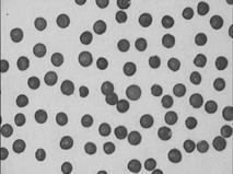
20 Classifi cation Introduction When objects are detected with suitable operators and their shape is described (Chapter 19), image processing has reached its goal for certain classes of applications. For other applications, further tasks remain to be solved. In this introduction we explore several examples which illustrate how the image processing tasks depend on the questions we pose. In many image processing applications, the size and shape of parti- cles such as bubbles, aerosols, drops, pigment particles, or cell nuclei must be analyzed. In these cases, the parameters of interest are clearly defi ned and directly measurable from the images taken. We determine the area and shape of each particle detected with the methods discussed in Sections 19.5.1 and 19.3. Knowing these parameters allows all the questions of interest to be answered. From the data collected, we can, for example, compute histograms of the particle area (Fig. 20.1c). This example is typical for a wide class of scientifi c applications. Object para- meters that can be evaluated directly and unambiguously from the image data help to answer the scientifi c questions asked. Other applications are more complex in the sense that it is required to distinguish diff erent classes of objects in an image. The easiest case is given by a typical industrial inspection task. Are the dimensions of a part within the given tolerance? Are any parts missing? Are any defects such as scratches visible? As the result of the analysis, the inspected part either passes the test or is assigned to a certain error class. Assigning objects in images to certain classes is — like many other as- pects of image processing and analysis — a truly interdisciplinary prob- lem which is not specifi c to image analysis but a very general type of technique. In this respect, image analysis is part of a more general re- search area known as pattern recognition. A classical application of pat- tern recognition that everybody knows is speech recognition. The spoken words are contained in a 1-D acoustic signal (a time series). Here, the classifi cation task is to recognize the phonemes, words, and sentences from the spoken language. The corresponding task in image processing is text recognition, the recognition of letters and words from a written text, also known as optical character recognition (OCR). A general diffi culty of classifi cation is related to the fact that the relationship between the parameters of interest and the image data is 513 B. Jä hne, Digital Image Processing Copyright © 2002 by Springer-Verlag ISBN 3–540–67754–2 All rights of reproduction in any form reserved. 514 20 Classifi cation
A b
c
25
15 10 5 0 0 500 1000 1500 2000
Figure 20.1: Steps to analyze the size distribution of particles (lentils): a original image, b binary image, and c area distribution.
not evident. The objects to be classifi ed are not directly related to a certain range of values of a single feature but have to be identifi ed by their optical signature in the image. By which features, for example, can we distinguish the lentils, peppercorns, and sunfl ower seeds shown in Fig. 20.2? The relation between the optical signatures and the object classes generally requires a careful investigation. We illustrate the com- plex relations between object features and their optical signatures with two further examples. “Waldsterben” (large-scale forest damage by acid rain and other envi- ronmental pollution) is one of the many large problems environmental scientists are faced with. In remote sensing, the task is to map and clas- sify the extent of the damage in forests from aerial and satellite imagery. In this example, the relationship between the diff erent classes of dam- age and features in the images is less evident. Detailed investigations are necessary to reveal these complex relationships. Aerial images must be compared with investigations on the ground. We can expect to need more than one feature to identify certain classes of forest damage. There are many similar applications in medical and biological science. One of the standard questions in medicine is to distinguish between “healthy” and “diseased”. Again, it is obvious that we cannot expect a 20.1 Introduction 515
A b
Figure 20.2: Classifi cation task: which of the seeds is a peppercorn, a lentil, a sunfl ower seed or none of the three? a Original image, and b binary image after segmentation.
simple relationship between these two object classes and features of the observed objects in the images. Take as another example the objects shown in Fig. 20.3. We will have no problem in recognizing that all objects but one are lamps. How could a machine vision system perform this task? What features can we extract from these images that help us recognize a lamp? While we have no problems in recognizing the lamps in Fig. 20.3, we feel quite helpless with the question as how we can solve this task using a computer. Obviously this task is complex. We recognize a lamp because we have already seen many other lamps before and somehow memorized this experience and are able to compare this stored knowledge with what we see in the image. But how is this knowledge stored and how is the comparison performed? It is obviously not just a database with geometric shapes, we also know in which context or environment lamps occur and for what they are used. Research on problems of this kind is part of a research area called artifi cial intelligence, abbreviated as AI. With respect to scientifi c applications, another aspect of classifi ca- tion is of interest. As imaging techniques are among the driving forces of progress in experimental natural sciences, it often happens that un- known objects appear in images, for which no classifi cation scheme is available so far. It is one goal of image processing to fi nd out possible classes for these new objects. Therefore, we need classifi cation tech- niques that do not require any previous knowledge. Summing up, we conclude that classifi cation includes two basic tasks: 1. The relation between the image features (optical signature) and the object classes sought must be investigated in as much detail as pos- sible. This topic is partly comprised in the corresponding scientifi c 516 20 Classifi cation
Figure 20.3: How do we recognize that all but one of these objects are lamps?
area and partly in image formation, i. e., optics, as discussed in Chap- ters 6–8. 2. From the multitude of possible image features, we must select an optimal set which allows the diff erent object classes to be distin- guished unambiguously with minimum eff ort and as few errors as possible by a suitable classifi cation technique. This task, known as classifi cation, is the topic of this chapter. We touch here only some basic questions such as selecting the proper type and number of fea- tures (Section 20.2) and devise some simple classifi cation techniques (Section 20.3).
Feature Space 20.2.1 Pixel-Based Versus Object-Based Classifi cation Two types of classifi cation procedures can be distinguished: pixel-based classifi cation and object-based classifi cation. In complex cases, a segmen- tation of objects is not possible using a single feature. Then it is already required to use multiple features and a classifi cation process to decide which pixel belongs to which type of object. 20.2 Feature Space 517
A much simpler object-based classifi cation can be used if the diff er- ent objects can be well separated from the background and do not touch or overlap each other. Object-based classifi cation should be used if at all possible, since much less data must be handled. Then all the pixel-based features discussed in Chapters 11–15, such as the mean gray value, local orientation, local wave number, and gray value variance, can be averaged over the whole area of the object and used as features describing the object’s properties. In addition, we can use all the parameters describ- ing the shape of the objects discussed in Chapter 19. Sometimes it is required to apply both classifi cation processes: fi rst, a pixel-based clas- sifi cation to separate the objects from each other and the background and, second, an object-based classifi cation to utilize also the geometric properties of the objects for classifi cation.
Cluster A set of P features forms a P-dimensional space M, denoted as a fea- ture space or measurement space. Each pixel or object is represented as a feature vector in this space. If the features represent an object class well, all feature vectors of the objects from this class should lie close to each other in the feature space. We regard classifi cation as a statis- tical process and assign a P-dimensional probability density function to each object class. In this sense, we can estimate this probability func- tion by taking samples from a given object class, computing the feature vector, and incrementing the corresponding point in the discrete feature space. This procedure is that of a generalized P-dimensional histogram (Section 3.2.1). When an object class shows a narrow probability distri- bution in the feature space, we speak of a cluster. It will be possible to separate the objects into given object classes if the clusters for the diff er- ent object classes are well separated from each other. With less suitable features, the clusters overlap each other or, even worse, no clusters may exist at all. In these cases, an error-free classifi cation is not possible.
Feature Selection We start with an example, the classifi cation of the diff erent seeds shown in Fig. 20.2 into the three classes peppercorns, lentils, and sunfl ower seeds. Figure 20.4a, b shows the histograms of the two features area and eccentricity (Eq. (19.6) in Section 19.3.3). While the area histogram shows two peaks, only one peak can be observed in the histogram of the eccentricity. In any case, neither of the two features alone is suffi cient to distinguish the three classes peppercorns, lentils, and sunfl ower seeds. If we take both parameters together, we can identify at least two clusters (Fig. 20.4c). These two classes can be identifi ed as the peppercorns and the lentils. Both seeds are almost circular and thus show a low eccen- 518 20 Classifi cation
A b
25 25
15 15 10 10 5 5
eccentricity 0 0 500 1000 1500 2000 0 0 0.2 0.4 0.6 0.8 1
0.8
0.4
0.2
0 0 200 400 600 800 1000 1200
Figure 20.4: Features for the classifi cation of diff erent seeds from Fig. 20.2 into peppercorns, lentils, and sunfl ower seeds: histogram of the features a area and b eccentricity; c two-dimensional feature space with both features.
tricity between 0 and 0.2. Therefore, both classes coalesce into one peak in the eccentricity histogram (Fig. 20.4b). The sunfl ower seeds do not form a dense cluster since they vary signifi cantly in shape and size. But it is obvious that they can be similar in size to the lentils. Thus it is not suffi cient to use only the feature area. In Figure 20.4c we can also identify several outliers. First, there are several small objects with high eccentricity. These are objects that are only partly visible at the edges of the image (Fig. 20.2). There are also fi ve large objects where touching lentils merge into larger objects. The eccentricity of these objects is also large and it may be impossible to distinguish them from sunfl ower seeds using the two simple parameters area and eccentricity only. The quality of the features is critical for a good classifi cation. What does this mean? At fi rst glance, we might think that as many features as possible would be the best solution. Generally, this is not the case. Figure 20.5a shows a one-dimensional feature space with three object 20.2 Feature Space 519 A b
m1 m1
Figure 20.5: a One-dimensional feature space with three object classes. b Exten- sion of the feature space with a second feature. The gray shaded areas indicate the regions in which the probability for a certain class is larger than zero. The same object classes are shown in a and b.
classes. The features of the fi rst and second class are separated, while those of the second and third class overlap considerably. A second fea- ture does not necessarily improve the classifi cation, as demonstrated in Fig. 20.5b. The clusters of the second and third class are still overlaid. A closer examination of the distribution in the feature space explains why: the second feature does not tell us much new. It varies in strong correlation with the fi rst feature. Thus, the two features are strongly correlated. Two additional basic facts are worth mentioning. It is often over- looked how many diff erent classes can be separated with a few parame- ters. Let us assume that one feature can only separate two classes. Then, ten features can separate 210 = 1024 object classes. This simple example illustrates the high separation potential of just a few parameters. The essential problem is the even distribution of the clusters in the feature space. Consequently, it is important to fi nd the right features, i. e., to study the relationship between the features of the objects and those in the images carefully.
|
Последнее изменение этой страницы: 2019-05-04; Просмотров: 207; Нарушение авторского права страницы


 p = ne + √ 2no, (19.18)

 30
30 20
20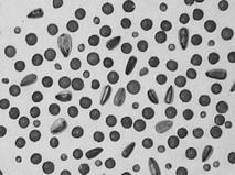


 0.6
0.6


