Chapter 1. Known formulas of the theory of matrices for ordinary differential equations.

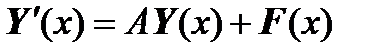
All methods are given by the example of a system of differential equations of the cylindrical shell of a rocket - a system of ordinary differential equations of the 8th order (after the separation of partial derivatives by Fourier’s method).

The system of linear ordinary differential equations has the form:

,

where  – the required vector-valued function of the dimension 8х1,  – the derivative of the required vector-valued function of the dimension 8х1,  – square matrix of coefficients of a differential equation of dimension 8х8,  – vector-function of external action on the system of dimension 8х1.

Hereinafter, vectors are denoted by boldface instead of dashes over letters.

The boundary value conditions have the form:

where  – the value of the required vector-function on the left-hand side x = 0 of dimension 8x1,  – rectangular horizontal matrix of coefficients of boundary conditions of the left edge of dimension 4х8,  – vector of external influences on the left edge of dimension 4х1,

 – the value of the required vector-function on the right-hand side x = 1 of dimension 8x1, – rectangular horizontal matrix of coefficients of the boundary conditions of the right edge of dimension 4х8,  – vector of external actions on the right edge of dimension 4х1.

In the case when the system of differential equations has a matrix with constant coefficients = const, the solution of Cauchy’s problem has the form [Gantmakher]:

,

 

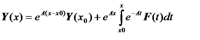where , where - is the unit matrix.

The matrix exponent can still be called Cauchy’s matrix and can be written as:

.

Then the solution of Cauchy’s problem can be written in the form:

,

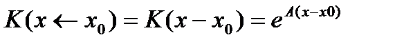where   is the vector of a particular solution of an inhomogeneous system of differential equations.

From the theory of matrices [Gantmakher], the property of multiplication of matrix exponentials (Cauchy’s matrices) is known:

In the case when the system of differential equations has a matrix with variable coefficients , the solution of Cauchy’s problem is proposed, as is known, to be sought using the property of multiplication of Cauchy’s matrices. That is, the interval of integration is divided into small sections and in small parts Cauchy’s matrix approximately calculated by the formula for the constant matrix in the exponent. And then Cauchy’s matrices calculated on small sections are multiplied:

,

where Cauchy’s matrices are approximately computed by the formula:

, где .

 

 

Chapter 2. Improvement of S.K.Godunov’s method of orthogonal sweep for solving boundary value problems with stiff ordinary differential equations.

⇐ Предыдущая123456789Следующая ⇒

Поделиться: