
|
Архитектура Аудит Военная наука Иностранные языки Медицина Металлургия Метрология Образование Политология Производство Психология Стандартизация Технологии |
|
|
Архитектура Аудит Военная наука Иностранные языки Медицина Металлургия Метрология Образование Политология Производство Психология Стандартизация Технологии |
Modification of S.K.Godunov’s sweep method.
The solution in S.K.Godunov’s method is sought, as written above, in the form of the formula
We can write this formula in two versions - in one case the formula satisfies the boundary conditions of the left edge (index L), and in the other - the conditions on the right edge (index R):
At an arbitrary point we have
Then we obtain
That is, a system of linear algebraic equations of the traditional kind with a square matrix of coefficients
Chapter 3. The method of "transferring of boundary value conditions" (the direct version of the method) for solving boundary value problems with non-stiff ordinary differential equations.
It is proposed to integrate by the formulas of the theory of matrices [Gantmakher] immediately from some inner point of the interval of integration to the edges:
We substitute the formula for
Similarly, for the right boundary conditions, we obtain:
That is, we obtain two matrix equations of boundary conditions transferred to the point
These equations are similarly combined into one system of linear algebraic equations with a square matrix of coefficients to find the solution
Chapter 4. The method of "additional boundary value conditions" for solving boundary value problems with non-stiff ordinary differential equations. Let us write on the left edge one more equation of the boundary conditions:
As matrix That is, for example, if the problem of the shell of a rocket is considered, then on the left edge 4 movements can be specified. Then for the matrix The vector
that is, the vector Similarly, we write on the right edge one more equation of the boundary conditions:
where the matrix For the right edge, too, the corresponding system of equations is valid:
We write
We write the vector
and substitute it in the previous formula:
Thus, we have obtained a system of equations of the form:
where the matrix We divide the matrix
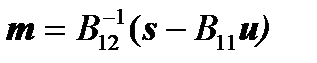
from which we can write that
Consequently, the required vector
And the required vector
Chapter 5. The method of "half of the constants" for solving boundary value problems with non-stiff ordinary differential equations.
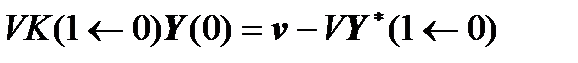
In this method we use the idea proposed by S.K.Godunov to seek a solution in the form of only one-half of the possible unknown constants, but a formula for the possibility of starting such a calculation and further application of matrix exponents (Cauchy’s matrices) are proposed by A.Yu.Vinogradov. The formula for starting calculations from the left edge with only one half of the possible constants:
Thus, a formula is written in the matrix form for the beginning of the calculation from the left edge, when the boundary conditions are satisfied on the left edge. Then write
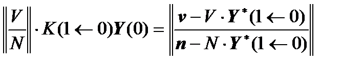
and substitute in this formula the expression for Y(0):
or
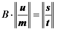
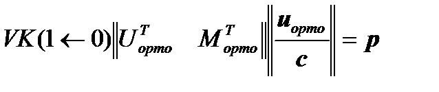
Thus, we have obtained an expression of the form:
where the matrix
Then we can write:
Hence we obtain that:
Thus, the required constants are found.
Chapter 6. The method of "transferring of boundary conditions" (step-by-step version of the method) for solving boundary value problems with stiff ordinary differential equations. 6.1. The method of "transfer of boundary value conditions" to any point of the interval of integration. The complete solution of the system of differential equations has the form
Or you can write:
We substitute this expression for
Or we get the boundary conditions transferred to the point
where Further, we write similarly
And substitute this expression for
Or we get the boundary conditions transferred to the point
where And so we transfer the matrix boundary condition from the left edge to the point Let us show the steps of transferring the boundary conditions of the right edge. We can write:
We substitute this expression for
Or we get the boundary conditions of the right edge, transferred to the point
where Further, we write similarly
And substitute this expression for
Or we get the boundary conditions transferred to the point
where And so at the inner point
From these two matrix equations with rectangular horizontal coefficient matrices, we obviously obtain one system of linear algebraic equations with a square matrix of coefficients:
6.2. The case of "stiff" differential equations. In the case of "stiff" differential equations, it is proposed to apply a line orthonormalization of the matrix boundary conditions in the process of their transfer to the point under consideration. For this, the orthonormalization formulas for systems of linear algebraic equations can be taken in [Berezin, Zhidkov]. That is, having received
we apply a line orthonormation to this group of linear algebraic equations and obtain an equivalent matrix boundary condition:
And in this line orthonormal equation is substituted
And we get
Or we get the boundary conditions transferred to the point
where Now we apply linear orthonorming to this group of linear algebraic equations and obtain an equivalent matrix boundary condition:
And so on. And similarly we do with intermediate matrix boundary conditions carried from the right edge to the point under consideration. As a result, we obtain a system of linear algebraic equations with a square matrix of coefficients, consisting of two independently stepwise orthonormal matrix boundary conditions, which is solved by Gauss’ method with the separation of the main element for obtaining the solution
|
Последнее изменение этой страницы: 2019-06-10; Просмотров: 166; Нарушение авторского права страницы
 .
. ,
, .
. .
. ,
, ,
, .
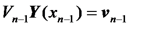
. for the computation of the vectors of constants
  is obtained.
  ,
, .
. in the boundary conditions of the left edge and obtain:
 ,
, ,
, .
. ,
, ,
, .
. under consideration:
 ,
, .
. at any point
 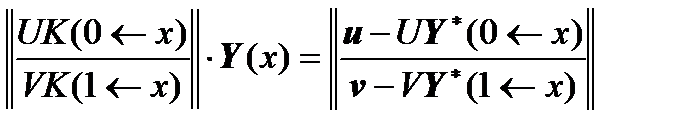 .
. .
. rows, we can take those boundary conditions, that is, expressions of those physical parameters that do not enter into the parameters of the boundary conditions of the left edge
  or are linearly independent with them. This is entirely possible, since for boundary value problems there are as many independent physical parameters as the dimensionality of the problem, and only half of the physical parameters of the problem enter into the parameters of the boundary conditions.
 we can take the parameters of forces and moments, which are also 4, since the total dimension of such a problem is 8.
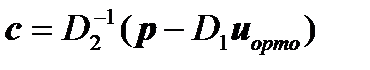
 of the right side is unknown and it must be found, and then we can assume that the boundary value problem is solved, that is, reduced to Cauchy’s problem, that is, the vector
  is found from the expression:
 ,
, .
. ,
, is written from the same considerations for additional linearly independent parameters on the right edge, and the vector
  is unknown.
 .
. and substitute it into the last system of linear algebraic equations:
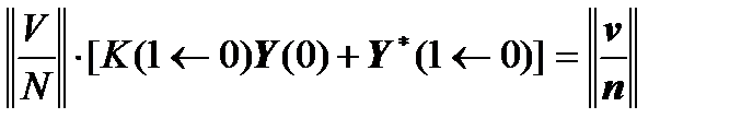 ,
, ,
, ,
, .
. through the inverse matrix:

 ,
, is known, the vectors
  and
and  are known, and the vectors
  and
and  are unknown.
 ,
,
 is calculated through the vector
  ,
, .
. ,
, .
. and
and  collectively:
 ,
,

 .
. ,
, has a dimension of 4x8 and can be naturally represented in the form of two square blocks of 4x4 dimension:
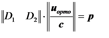 .
. .
. .
. .
. .
. into the boundary conditions of the left edge and obtain:
 ,
, ,
, .
. :
: ,
, and
and  .
.
 into the transferred boundary conditions of the point
  :
: ,
, ,
, .
. :
: ,
, and
and  .
. and in the same way transfer the matrix boundary condition from the right edge.
 in the boundary conditions of the right edge and obtain:
 ,
, ,
,
 :
: ,
, and
and  .
.
 in the transferred boundary conditions of the point
  :
: ,
, .
. :
: ,
, and
and 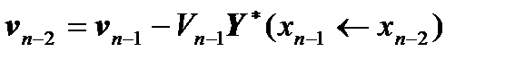 .
. ,
, .
. .
. .
. .
. ,
, .
. and
and  .
.
 at the point
  under consideration:
 .
.