Applicable formulas for orthonormalization.

Taken from [Berezin, Zhidkov]. Let there be given a system of linear algebraic equations of order n:

= .

 

Here, above the vectors, we draw dashes instead of their designation in boldface.

We will consider the rows of the matrix  of the system as vectors:

=( , ,…, ).

 

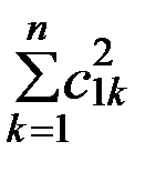
We orthonormalize this system of vectors.

The first equation of the system =  we divide by .

In doing so, we get:

+ +…+ = , =( , ,…, ),

where = , = , =1.

 

The second equation of the system is replaced by:

+ +…+ = , =( , ,…, ),

where = , = ,

= -( , ) , = -( , ) .

 

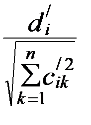
Similarly we proceed further. The equation with the number i takes the form:

+ +…+ = , =( , ,…, ),

where = , = ,

= -( , ) -( , ) -…-( , ) , 

= -( , ) -( , ) -…-( , ) .

 

Here ( , )  is the scalar multiplication of vectors.         

The process will be realized if the system of linear algebraic equations is linearly independent.

As a result, we come to a new system , where the matrix  will be with orthonormal rows, that is, it has the property , where  is the identity matrix.

 

 

Chapter 7. The simplest method for solving boundary value problems with stiff ordinary differential equations without orthonormalization - the method of "conjugation of sections of the integration interval", which are expressed by matrix exponents.

The idea of overcoming the difficulties of computation by dividing the interval of integration into conjugate areas belongs to Dr.Sc. Professor Yu.I.Vinogradov (his doctoral thesis was defended including on this idea), and the simplest realization of this idea through the formulas of the theory of matrices belongs to the Ph.D. A.Yu.Vinogradov.

We divide the interval of integration of the boundary value problem, for example, into 3 sections. We will have points (nodes), including edges:

.

We have boundary conditions in the form:

We can write the matrix equations of conjugation of sections:

,

,

.

We can rewrite it in a form more convenient for us further:

,

,

.

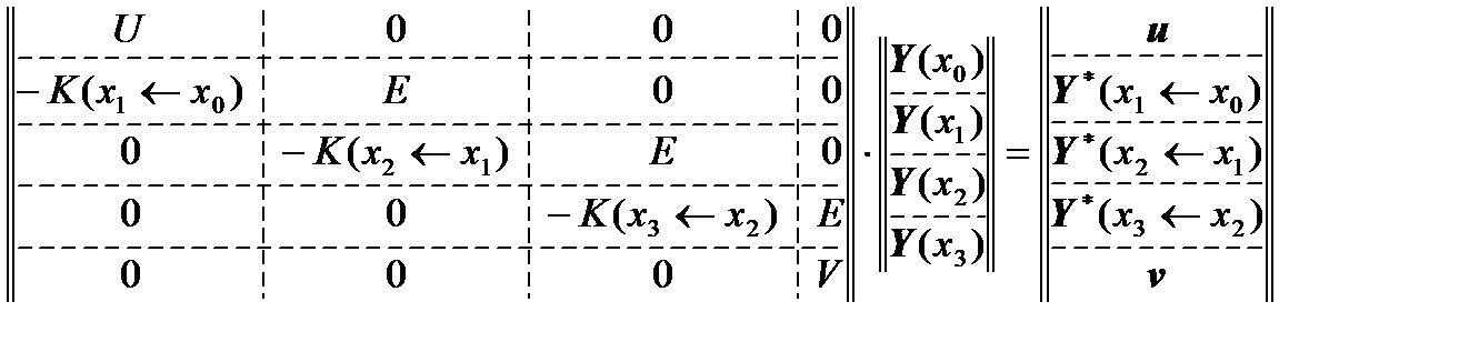
where  is the identity matrix.

Then in a combined matrix form we obtain a system of linear algebraic equations in the following form:

.

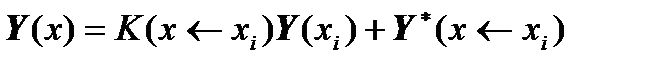
This system is solved by Gauss’ method with the separation of the main element.

At points located between nodes, the solution is to be solved by solving Cauchy’s problems with the initial conditions in the i-th node:

 

.

It is not necessary to apply orthonormalization for boundary value problems for stiff ordinary differential equations, since on each section of the integration interval the calculation of each matrix exponent is fulfilled independently and from the initial orthonormal identity matrix, which makes it unnecessary to use orthonormalization, unlike S.K.Godunov’s method, which greatly simplifies programming in comparison with S.K.Godunov's method.

It is possible to calculate Cauchy’s matrices not in the form of matrix exponents, but with Runge-Kutta’s methods from the starting identity matrix, and the vector of the particular solution of the inhomogeneous system of differential equations can be calculated on each site by Runge-Kutta’s methods from the starting zero vector. In the case of Runge-Kutta’s methods, error estimates are well known, which means that calculations can be performed with a known accuracy.

 

 

Chapter 8. Calculation of shells of composite and with frames by the simplest method of "conjugation of sections of the integration interval".

8.1. The variant of recording of the method for solving stiff boundary value problems without orthonormalization - the method of "conjugation of sections, expressed by matrix exponents "- with positive directions of matrix formulas of integration of differential equations.

We divide the interval of integration of the boundary value problem, for example, into 3 sections. We will have points (nodes), including edges:

.

We have boundary conditions in the form:

We can write the matrix equations of conjugation of sections:

,

,

.

We can rewrite it in a form more convenient for us further:

,

,

.

where  is the identity matrix.

As a result, we obtain a system of linear algebraic equations:

.

This system is solved by Gauss’ method with the separation of the main element.

It turns out that it is not necessary to apply orthonormalization, since sections of the integration interval are chosen so long that the computation on them is stable.

At points near the nodes, the solution is found by solving the corresponding Cauchy’s problems with the origin at the i-th node:

.

 

⇐ Предыдущая123456789Следующая ⇒

Поделиться: